Jittered points

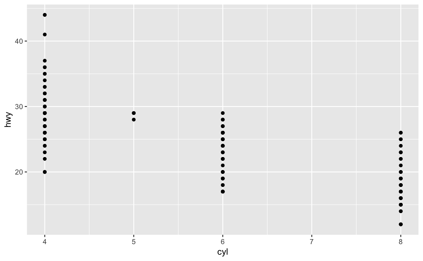
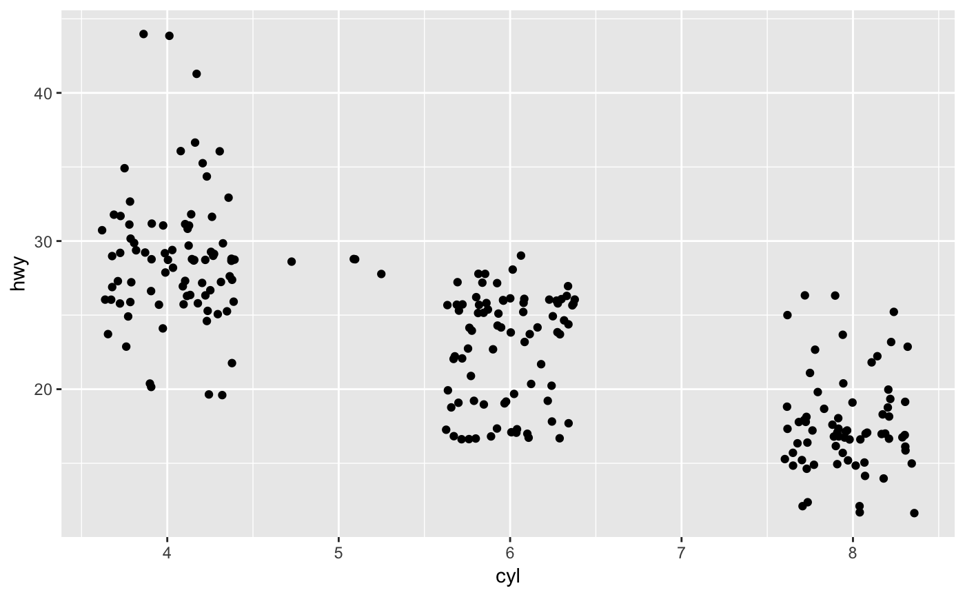
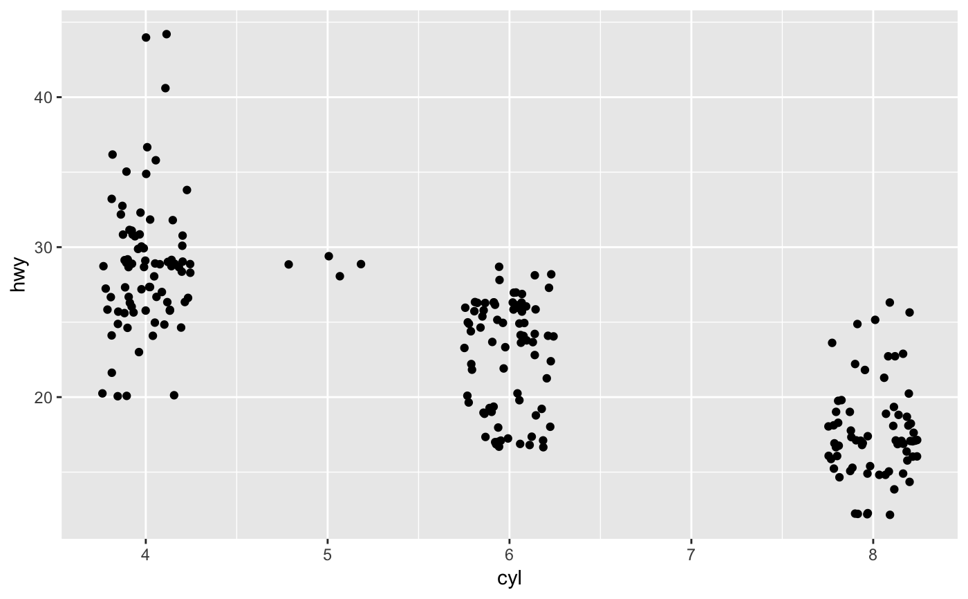
The jitter geom is a convenient shortcut for geom_point(position = "jitter"). It adds a small amount of random variation to the location of each point, and is a useful way of handling overplotting caused by discreteness in smaller datasets.

geom_jitter(mapping = NULL, data = NULL, stat = "identity",
  position = "jitter", ..., width = NULL, height = NULL, na.rm = FALSE,
  show.legend = NA, inherit.aes = TRUE)

Arguments

mapping	Set of aesthetic mappings created by aes() or aes_(). If specified and inherit.aes = TRUE (the default), it is combined with the default mapping at the top level of the plot. You must supply mapping if there is no plot mapping.
data	The data to be displayed in this layer. There are three options: If NULL, the default, the data is inherited from the plot data as specified in the call to ggplot(). A data.frame, or other object, will override the plot data. All objects will be fortified to produce a data frame. See fortify() for which variables will be created. A function will be called with a single argument, the plot data. The return value must be a data.frame., and will be used as the layer data.
stat	The statistical transformation to use on the data for this layer, as a string.
position	Position adjustment, either as a string, or the result of a call to a position adjustment function.
...	Other arguments passed on to layer(). These are often aesthetics, used to set an aesthetic to a fixed value, like color = "red" or size = 3. They may also be parameters to the paired geom/stat.
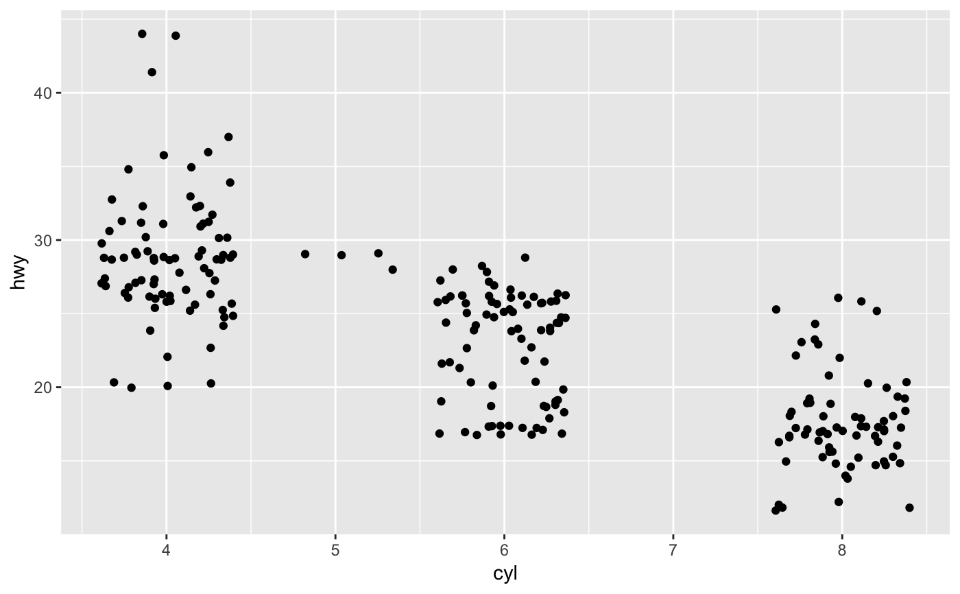
width	Amount of vertical and horizontal jitter. The jitter is added in both positive and negative directions, so the total spread is twice the value specified here. If omitted, defaults to 40% of the resolution of the data: this means the jitter values will occupy 80% of the implied bins. Categorical data is aligned on the integers, so a width or height of 0.5 will spread the data so it's not possible to see the distinction between the categories.
height	Amount of vertical and horizontal jitter. The jitter is added in both positive and negative directions, so the total spread is twice the value specified here. If omitted, defaults to 40% of the resolution of the data: this means the jitter values will occupy 80% of the implied bins. Categorical data is aligned on the integers, so a width or height of 0.5 will spread the data so it's not possible to see the distinction between the categories.
na.rm	If FALSE, the default, missing values are removed with a warning. If TRUE, missing values are silently removed.
show.legend	logical. Should this layer be included in the legends? NA, the default, includes if any aesthetics are mapped. FALSE never includes, and TRUE always includes. It can also be a named logical vector to finely select the aesthetics to display.
inherit.aes	If FALSE, overrides the default aesthetics, rather than combining with them. This is most useful for helper functions that define both data and aesthetics and shouldn't inherit behaviour from the default plot specification, e.g. borders().

Aesthetics

geom_point understands the following aesthetics (required aesthetics are in bold):

• x

• y

• alpha

• colour

• fill

• group

• shape

• size

• stroke

Learn more about setting these aesthetics in vignette("ggplot2-specs")

See also

geom_point() for regular, unjittered points, geom_boxplot() for another way of looking at the conditional distribution of a variable

Examples

p <- ggplot(mpg, aes(cyl, hwy))
p + geom_point()
p + geom_jitter()

# Add aesthetic mappings
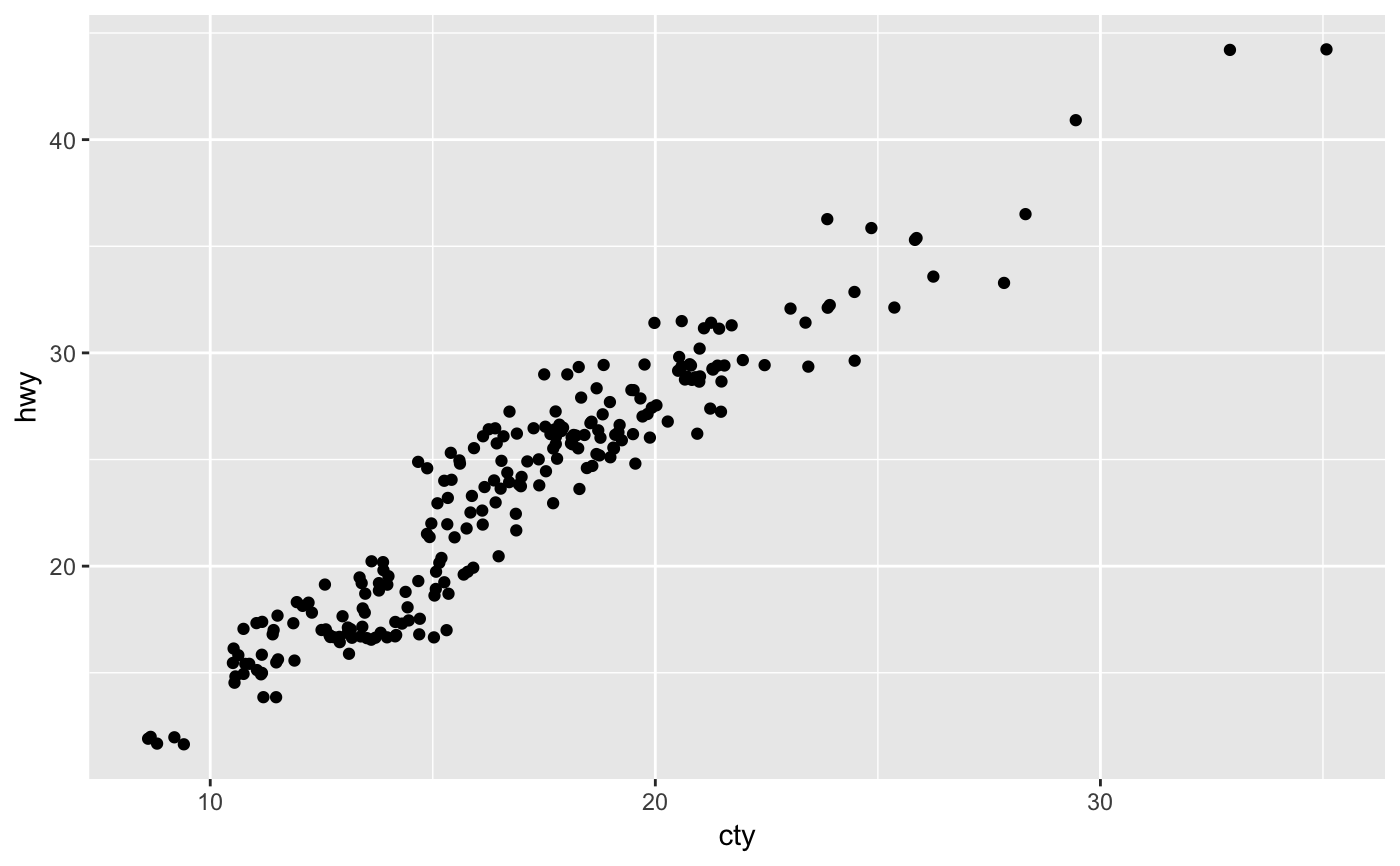
p + geom_jitter(aes(colour = class))

# Use smaller width/height to emphasise categories
ggplot(mpg, aes(cyl, hwy)) + geom_jitter()
ggplot(mpg, aes(cyl, hwy)) + geom_jitter(width = 0.25)

# Use larger width/height to completely smooth away discreteness
ggplot(mpg, aes(cty, hwy)) + geom_jitter()
ggplot(mpg, aes(cty, hwy)) + geom_jitter(width = 0.5, height = 0.5)