Set scale limits

This is a shortcut for supplying the limits argument to the individual scales. Note that, by default, any values outside the limits will be replaced with NA.

lims(...)

xlim(...)

ylim(...)

Arguments

...

A name-value pair. The name must be an aesthetic, and the value must be either a length-2 numeric, a character, a factor, or a date/time. A numeric value will create a continuous scale. If the larger value comes first, the scale will be reversed. You can leave one value as NA to compute from the range of the data. A character or factor value will create a discrete scale. A date-time value will create a continuous date/time scale.

See also

For changing x or y axis limits without dropping data observations, see coord_cartesian(). To expand the range of a plot to always include certain values, see expand_limits().

Examples

# Zoom into a specified area
ggplot(mtcars, aes(mpg, wt)) +
  geom_point() +
  xlim(15, 20)
#> Warning: Removed 19 rows containing missing values (geom_point).

# reverse scale
ggplot(mtcars, aes(mpg, wt)) +
  geom_point() +
  xlim(20, 15)
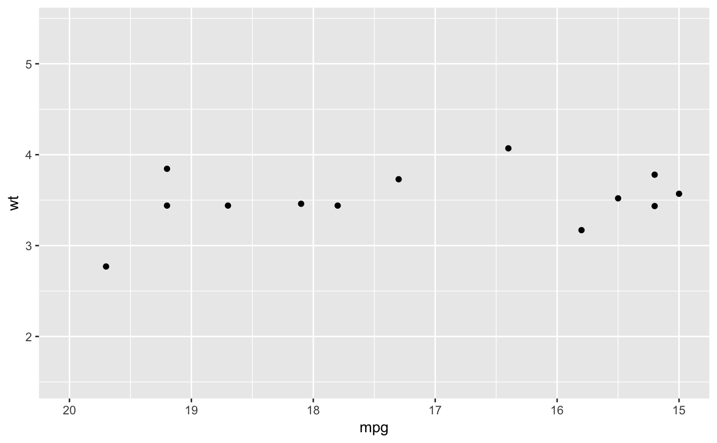
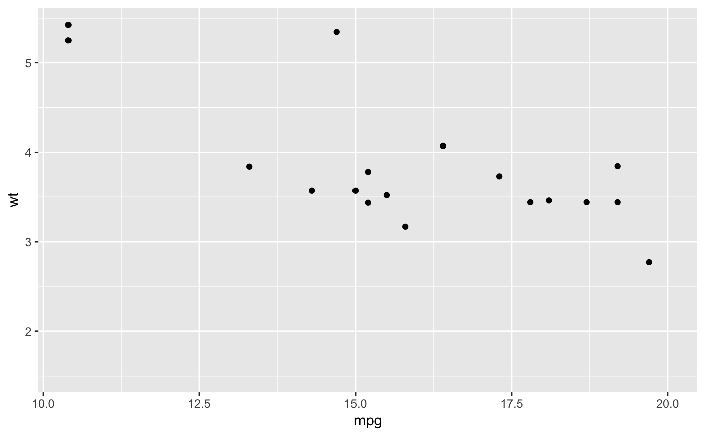
#> Warning: Removed 19 rows containing missing values (geom_point).

# with automatic lower limit
ggplot(mtcars, aes(mpg, wt)) +
  geom_point() +
  xlim(NA, 20)
#> Warning: Removed 14 rows containing missing values (geom_point).

# You can also supply limits that are larger than the data.
# This is useful if you want to match scales across different plots
small <- subset(mtcars, cyl == 4)
big <- subset(mtcars, cyl > 4)

ggplot(small, aes(mpg, wt, colour = factor(cyl))) +
  geom_point() +
  lims(colour = c("4", "6", "8"))

ggplot(big, aes(mpg, wt, colour = factor(cyl))) +
  geom_point() +
  lims(colour = c("4", "6", "8"))