Smoothed conditional means

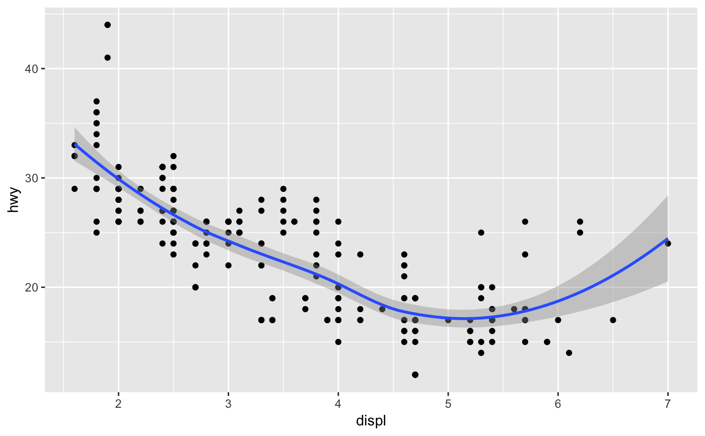
Aids the eye in seeing patterns in the presence of overplotting. geom_smooth and stat_smooth are effectively aliases: they both use the same arguments. Use geom_smooth unless you want to display the results with a non-standard geom.

geom_smooth(mapping = NULL, data = NULL, stat = "smooth",
  position = "identity", ..., method = "auto", formula = y ~ x,
  se = TRUE, na.rm = FALSE, show.legend = NA, inherit.aes = TRUE)

stat_smooth(mapping = NULL, data = NULL, geom = "smooth",
  position = "identity", ..., method = "auto", formula = y ~ x,
  se = TRUE, n = 80, span = 0.75, fullrange = FALSE, level = 0.95,
  method.args = list(), na.rm = FALSE, show.legend = NA,
  inherit.aes = TRUE)

Arguments

mapping	Set of aesthetic mappings created by aes() or aes_(). If specified and inherit.aes = TRUE (the default), it is combined with the default mapping at the top level of the plot. You must supply mapping if there is no plot mapping.
data	The data to be displayed in this layer. There are three options: If NULL, the default, the data is inherited from the plot data as specified in the call to ggplot(). A data.frame, or other object, will override the plot data. All objects will be fortified to produce a data frame. See fortify() for which variables will be created. A function will be called with a single argument, the plot data. The return value must be a data.frame., and will be used as the layer data.
position	Position adjustment, either as a string, or the result of a call to a position adjustment function.
...	Other arguments passed on to layer(). These are often aesthetics, used to set an aesthetic to a fixed value, like color = "red" or size = 3. They may also be parameters to the paired geom/stat.
method	Smoothing method (function) to use, eg. lm, glm, gam, loess, MASS::rlm. For method = "auto" the smoothing method is chosen based on the size of the largest group (across all panels). loess() is used for less than 1,000 observations; otherwise mgcv::gam() is used with formula = y ~ s(x, bs = "cs"). Somewhat anecdotally, loess gives a better appearance, but is O(n^2) in memory, so does not work for larger datasets. If you have fewer than 1,000 observations but want to use the same gam model that method = "auto" would use then set method = "gam", formula = y ~ s(x, bs = "cs").
formula	Formula to use in smoothing function, eg. y ~ x, y ~ poly(x, 2), y ~ log(x)
se	Display confidence interval around smooth? (TRUE by default, see level to control.)
na.rm	If FALSE, the default, missing values are removed with a warning. If TRUE, missing values are silently removed.
show.legend	logical. Should this layer be included in the legends? NA, the default, includes if any aesthetics are mapped. FALSE never includes, and TRUE always includes. It can also be a named logical vector to finely select the aesthetics to display.
inherit.aes	If FALSE, overrides the default aesthetics, rather than combining with them. This is most useful for helper functions that define both data and aesthetics and shouldn't inherit behaviour from the default plot specification, e.g. borders().
geom, stat	Use to override the default connection between geom_smooth and stat_smooth.
n	Number of points at which to evaluate smoother.
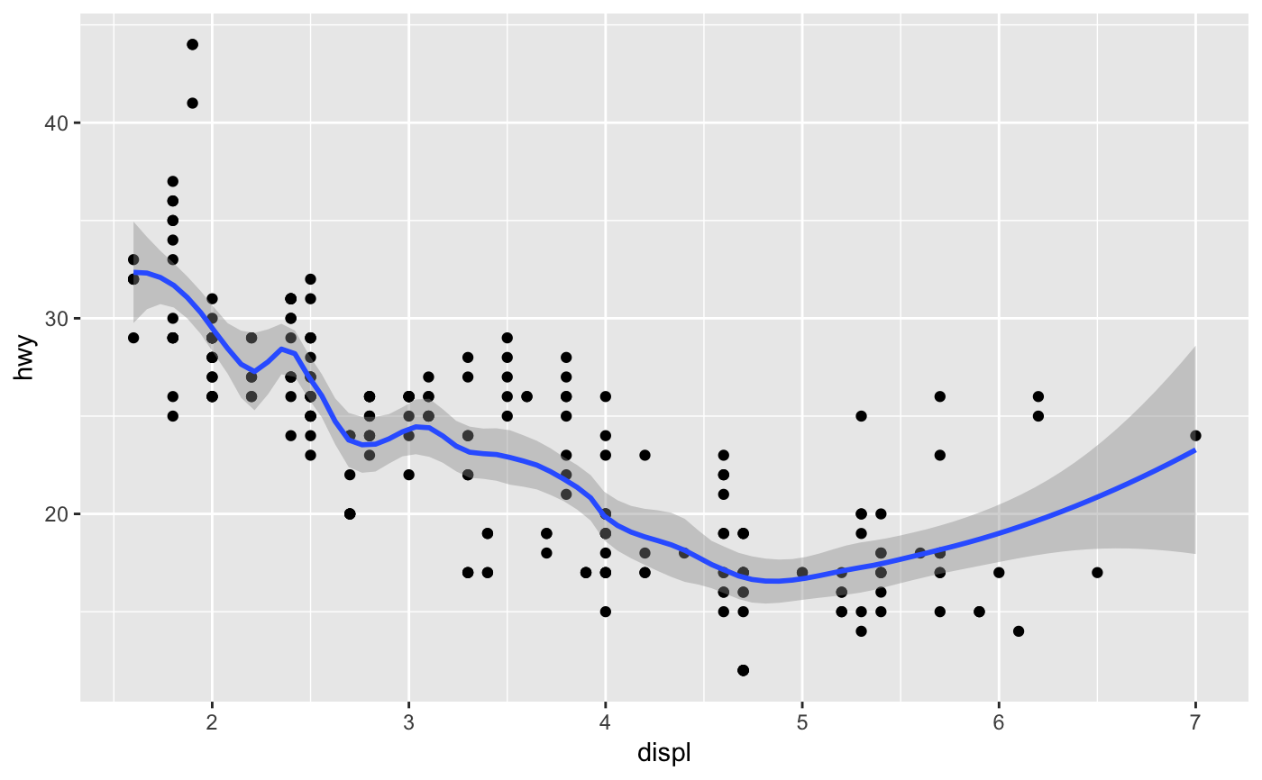
span	Controls the amount of smoothing for the default loess smoother. Smaller numbers produce wigglier lines, larger numbers produce smoother lines.
fullrange	Should the fit span the full range of the plot, or just the data?
level	Level of confidence interval to use (0.95 by default).
method.args	List of additional arguments passed on to the modelling function defined by method.

Details

Calculation is performed by the (currently undocumented) predictdf generic and its methods. For most methods the standard error bounds are computed using the predict() method - the exceptions are loess which uses a t-based approximation, and glm where the normal confidence interval is constructed on the link scale, and then back-transformed to the response scale.

Aesthetics

geom_smooth understands the following aesthetics (required aesthetics are in bold):

• x

• y

• alpha

• colour

• fill

• group

• linetype

• size

• weight

• ymax

• ymin

Learn more about setting these aesthetics in vignette("ggplot2-specs")

Computed variables

y

predicted value

ymin

lower pointwise confidence interval around the mean

ymax

upper pointwise confidence interval around the mean

se

standard error

See also

See individual modelling functions for more details: lm() for linear smooths, glm() for generalised linear smooths, loess() for local smooths

Examples

ggplot(mpg, aes(displ, hwy)) +
  geom_point() +
  geom_smooth()
#> `geom_smooth()` using method = 'loess' and formula 'y ~ x'

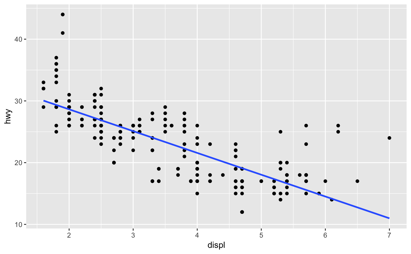
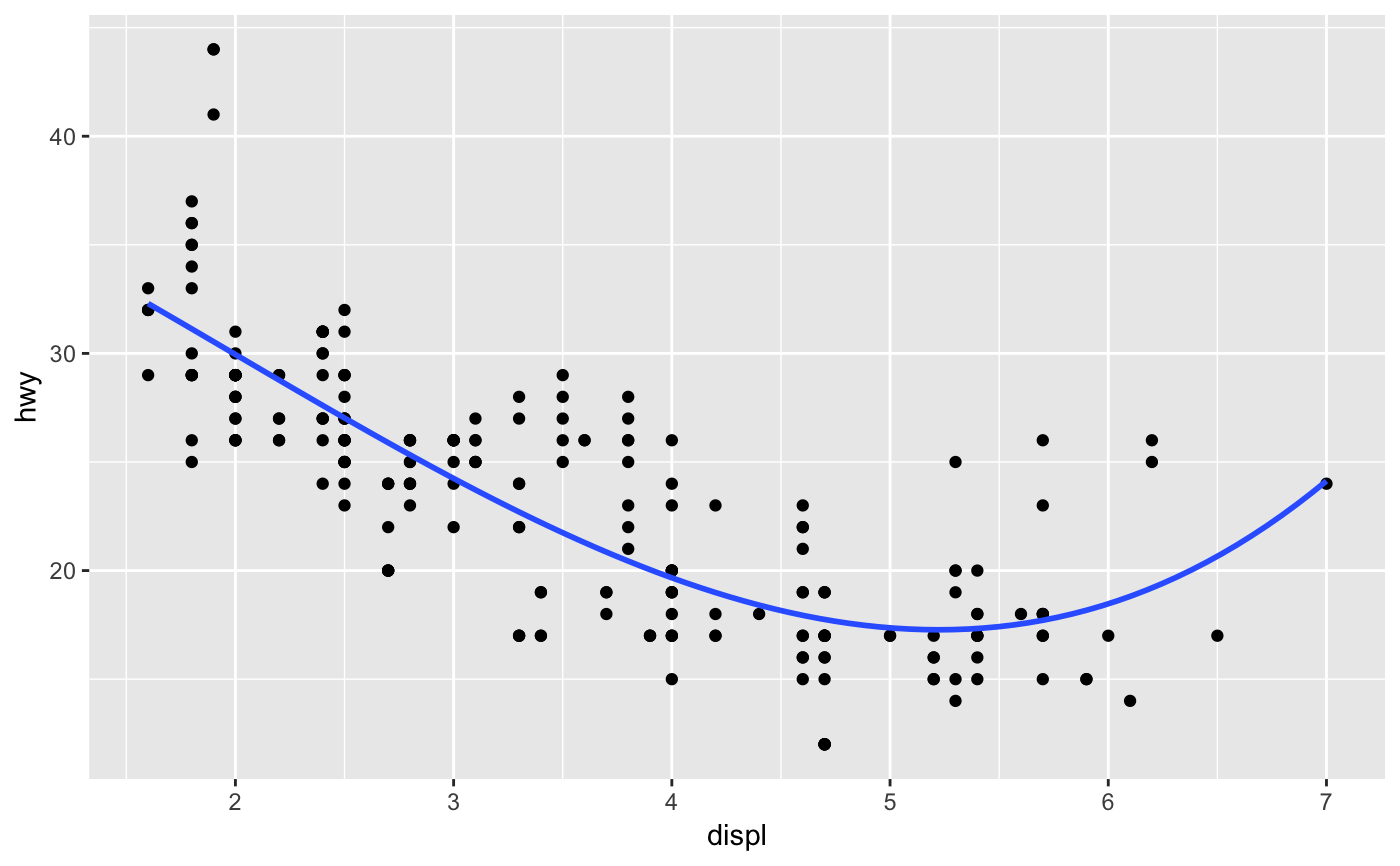
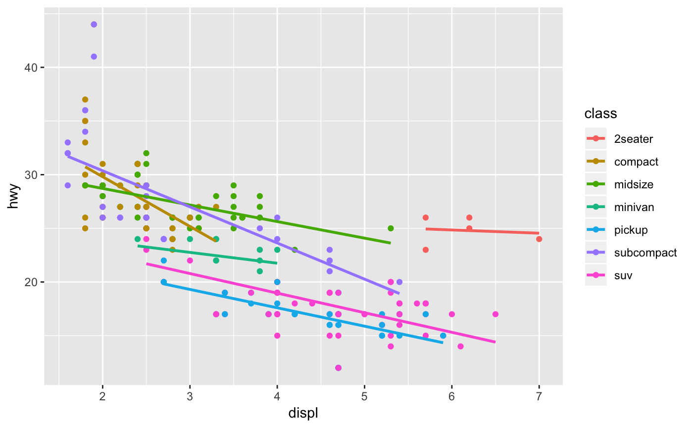
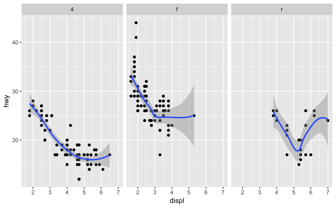
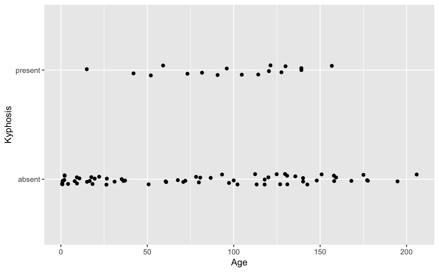
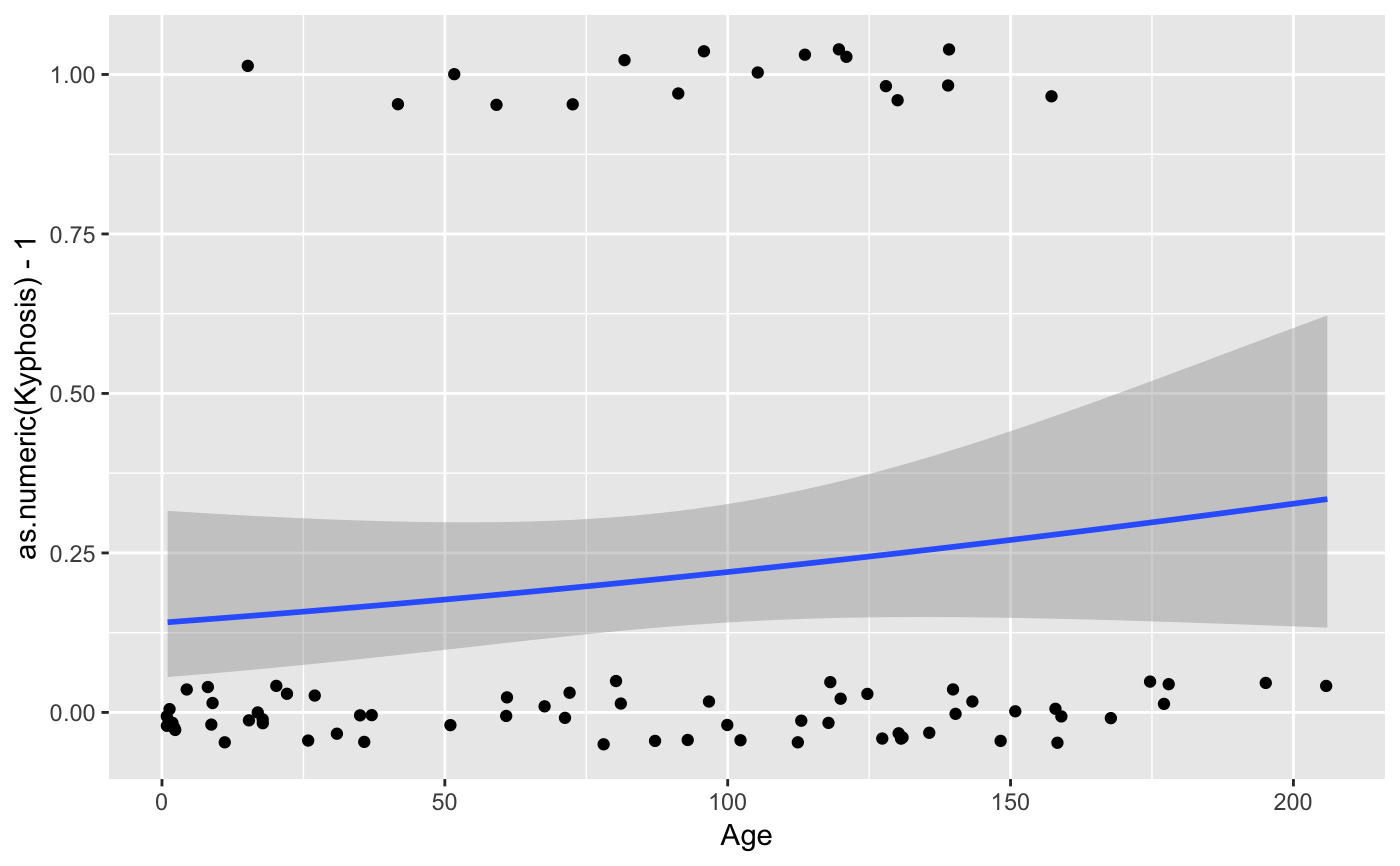
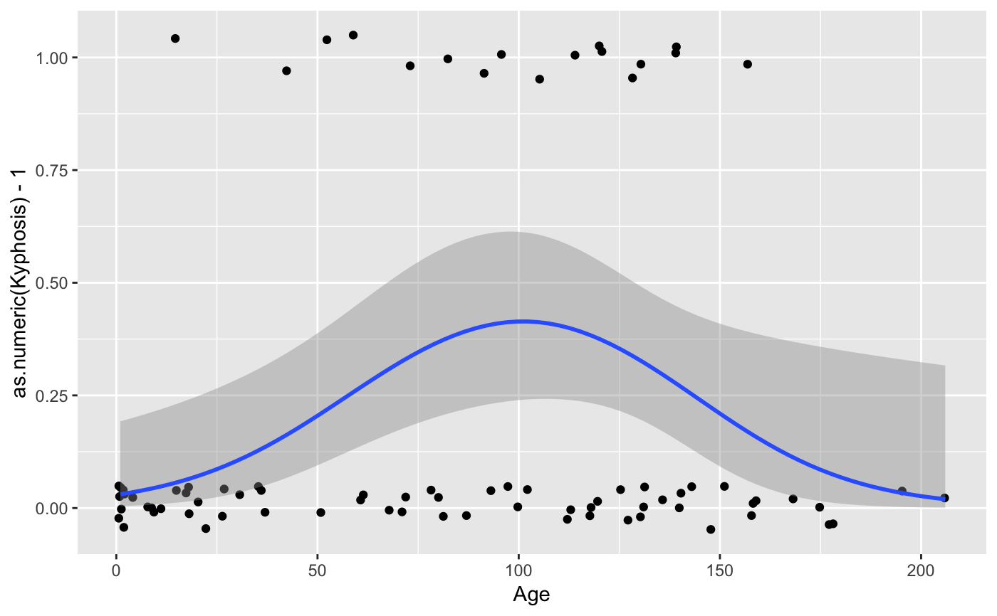
# Use span to control the "wiggliness" of the default loess smoother
# The span is the fraction of points used to fit each local regression:
# small numbers make a wigglier curve, larger numbers make a smoother curve.
ggplot(mpg, aes(displ, hwy)) +
  geom_point() +
  geom_smooth(span = 0.3)
#> `geom_smooth()` using method = 'loess' and formula 'y ~ x'

# Instead of a loess smooth, you can use any other modelling function:
ggplot(mpg, aes(displ, hwy)) +
  geom_point() +
  geom_smooth(method = lm, se = FALSE)

ggplot(mpg, aes(displ, hwy)) +
  geom_point() +
  geom_smooth(method = lm, formula = y ~ splines::bs(x, 3), se = FALSE)

# Smoothes are automatically fit to each group (defined by categorical
# aesthetics or the group aesthetic) and for each facet

ggplot(mpg, aes(displ, hwy, colour = class)) +
  geom_point() +
  geom_smooth(se = FALSE, method = lm)
ggplot(mpg, aes(displ, hwy)) +
  geom_point() +
  geom_smooth(span = 0.8) +
  facet_wrap(~drv)
#> `geom_smooth()` using method = 'loess' and formula 'y ~ x'

binomial_smooth <- function(...) {
  geom_smooth(method = "glm", method.args = list(family = "binomial"), ...)
}
# To fit a logistic regression, you need to coerce the values to
# a numeric vector lying between 0 and 1.
ggplot(rpart::kyphosis, aes(Age, Kyphosis)) +
  geom_jitter(height = 0.05) +
  binomial_smooth()
#> Warning: Computation failed in `stat_smooth()`:
#> y values must be 0 <= y <= 1

ggplot(rpart::kyphosis, aes(Age, as.numeric(Kyphosis) - 1)) +
  geom_jitter(height = 0.05) +
  binomial_smooth()

ggplot(rpart::kyphosis, aes(Age, as.numeric(Kyphosis) - 1)) +
  geom_jitter(height = 0.05) +
  binomial_smooth(formula = y ~ splines::ns(x, 2))

# But in this case, it's probably better to fit the model yourself
# so you can exercise more control and see whether or not it's a good model