Violin plot

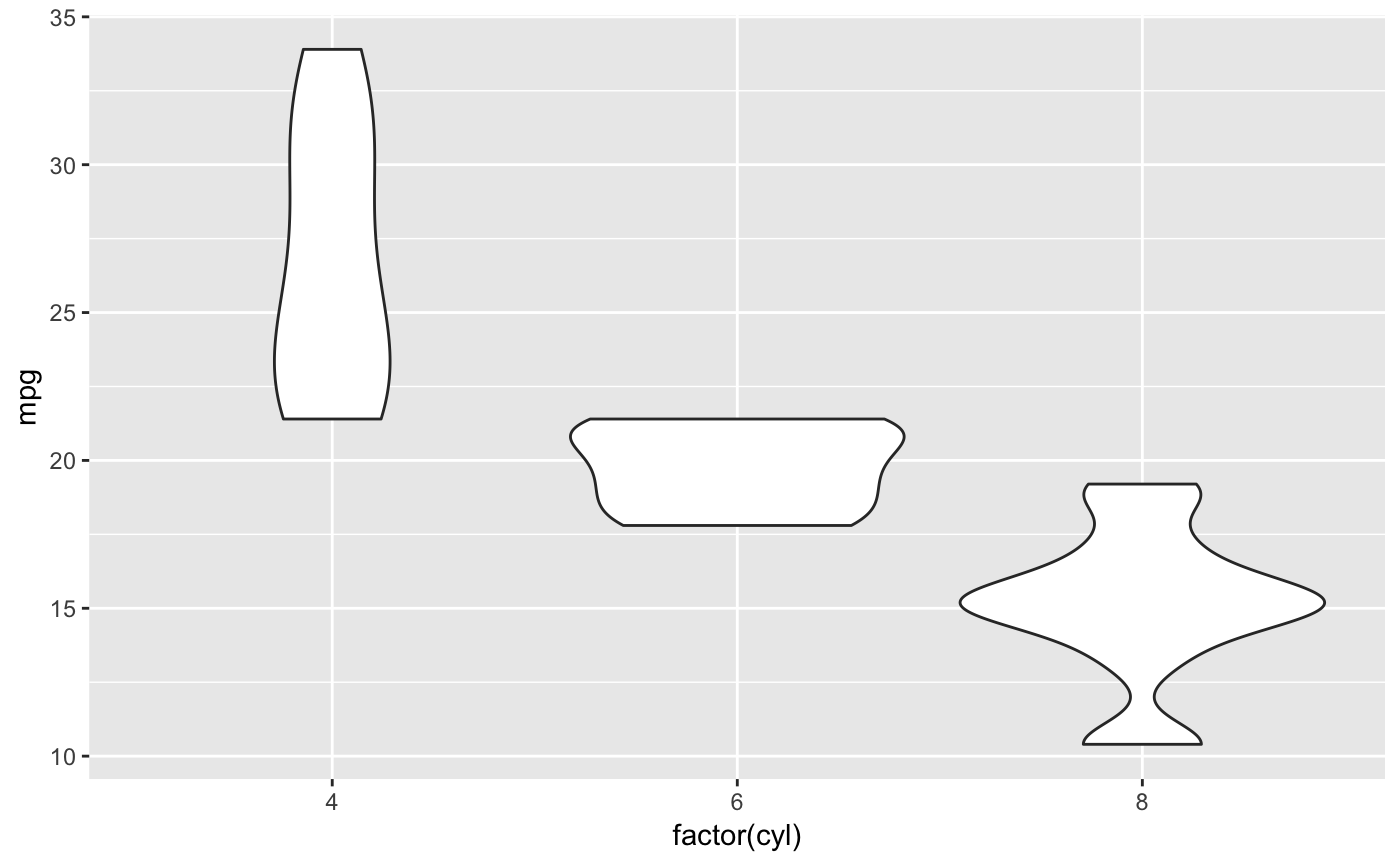
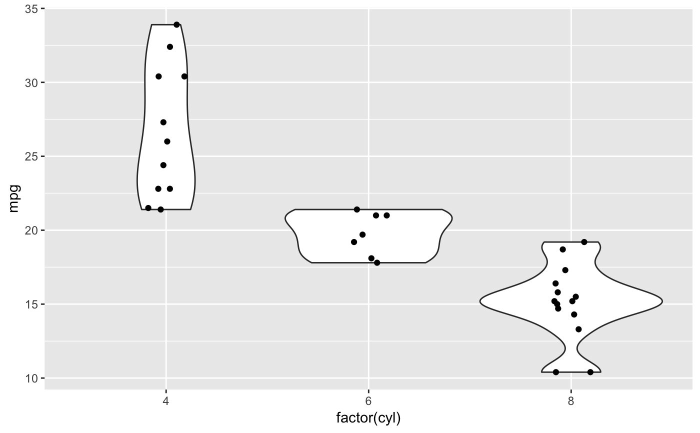
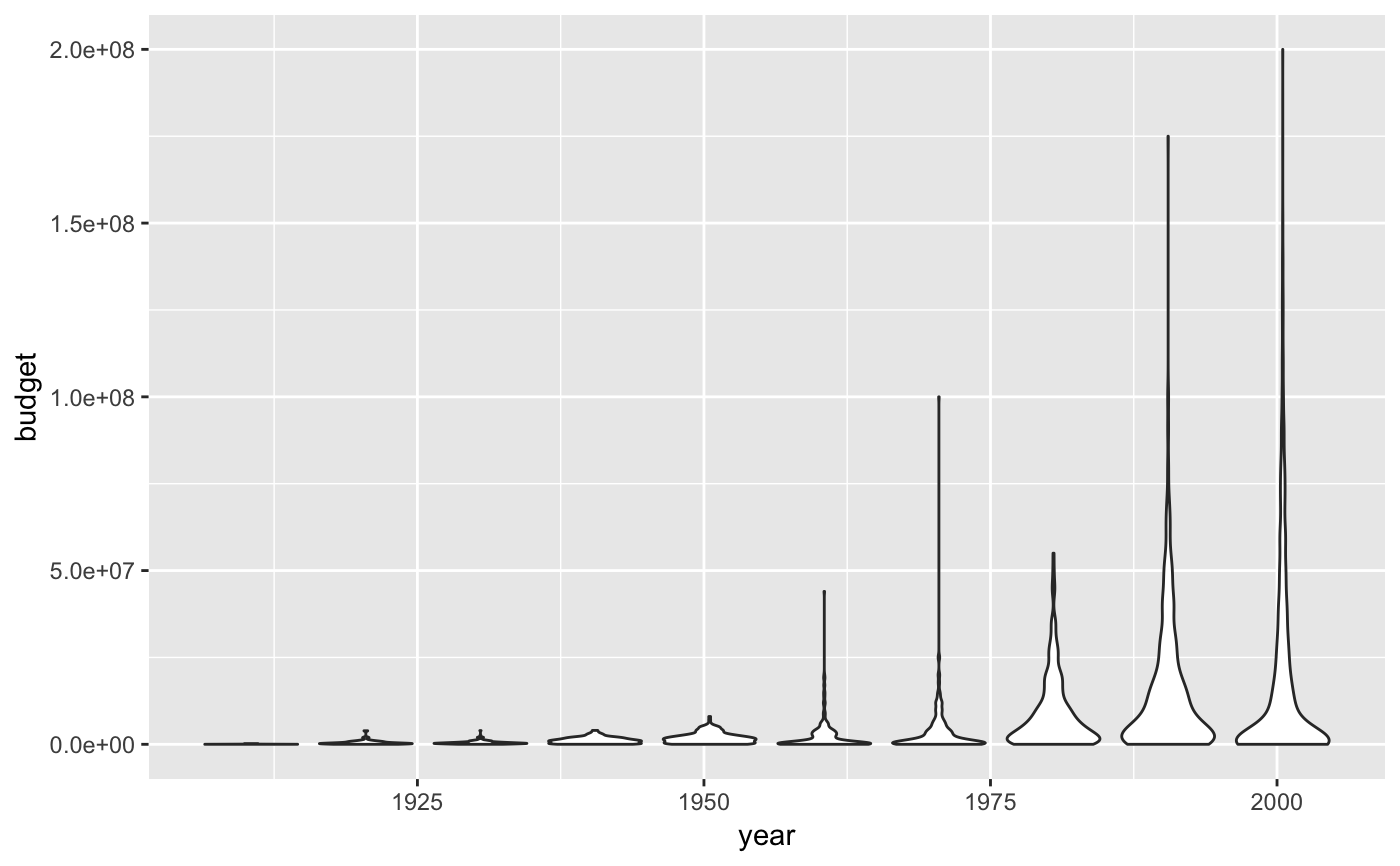
A violin plot is a compact display of a continuous distribution. It is a blend of geom_boxplot() and geom_density(): a violin plot is a mirrored density plot displayed in the same way as a boxplot.

geom_violin(mapping = NULL, data = NULL, stat = "ydensity",
  position = "dodge", ..., draw_quantiles = NULL, trim = TRUE,
  scale = "area", na.rm = FALSE, show.legend = NA, inherit.aes = TRUE)

stat_ydensity(mapping = NULL, data = NULL, geom = "violin",
  position = "dodge", ..., bw = "nrd0", adjust = 1, kernel = "gaussian",
  trim = TRUE, scale = "area", na.rm = FALSE, show.legend = NA,
  inherit.aes = TRUE)

Arguments

mapping	Set of aesthetic mappings created by aes() or aes_(). If specified and inherit.aes = TRUE (the default), it is combined with the default mapping at the top level of the plot. You must supply mapping if there is no plot mapping.
data	The data to be displayed in this layer. There are three options: If NULL, the default, the data is inherited from the plot data as specified in the call to ggplot(). A data.frame, or other object, will override the plot data. All objects will be fortified to produce a data frame. See fortify() for which variables will be created. A function will be called with a single argument, the plot data. The return value must be a data.frame., and will be used as the layer data.
position	Position adjustment, either as a string, or the result of a call to a position adjustment function.
...	Other arguments passed on to layer(). These are often aesthetics, used to set an aesthetic to a fixed value, like color = "red" or size = 3. They may also be parameters to the paired geom/stat.
draw_quantiles	If not(NULL) (default), draw horizontal lines at the given quantiles of the density estimate.
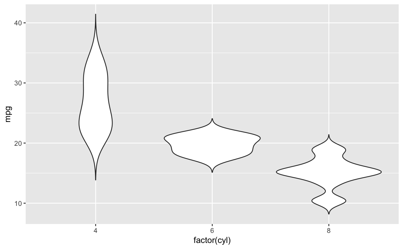
trim	If TRUE (default), trim the tails of the violins to the range of the data. If FALSE, don't trim the tails.
scale	if "area" (default), all violins have the same area (before trimming the tails). If "count", areas are scaled proportionally to the number of observations. If "width", all violins have the same maximum width.
na.rm	If FALSE, the default, missing values are removed with a warning. If TRUE, missing values are silently removed.
show.legend	logical. Should this layer be included in the legends? NA, the default, includes if any aesthetics are mapped. FALSE never includes, and TRUE always includes. It can also be a named logical vector to finely select the aesthetics to display.
inherit.aes	If FALSE, overrides the default aesthetics, rather than combining with them. This is most useful for helper functions that define both data and aesthetics and shouldn't inherit behaviour from the default plot specification, e.g. borders().
geom, stat	Use to override the default connection between geom_violin and stat_ydensity.
bw	The smoothing bandwidth to be used. If numeric, the standard deviation of the smoothing kernel. If character, a rule to choose the bandwidth, as listed in stats::bw.nrd().
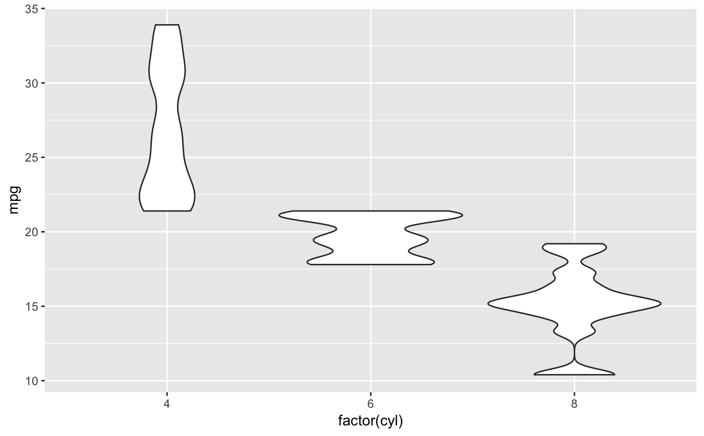
adjust	A multiplicate bandwidth adjustment. This makes it possible to adjust the bandwidth while still using the a bandwidth estimator. For example, adjust = 1/2 means use half of the default bandwidth.
kernel	Kernel. See list of available kernels in density().

Aesthetics

geom_violin understands the following aesthetics (required aesthetics are in bold):

• x

• y

• alpha

• colour

• fill

• group

• linetype

• size

• weight

Learn more about setting these aesthetics in vignette("ggplot2-specs")

Computed variables

density

density estimate

scaled

density estimate, scaled to maximum of 1

count

density * number of points - probably useless for violin plots

violinwidth

density scaled for the violin plot, according to area, counts or to a constant maximum width

n

number of points

width

width of violin bounding box

References

Hintze, J. L., Nelson, R. D. (1998) Violin Plots: A Box Plot-Density Trace Synergism. The American Statistician 52, 181-184.

See also

geom_violin() for examples, and stat_density() for examples with data along the x axis.

Examples

p <- ggplot(mtcars, aes(factor(cyl), mpg))
p + geom_violin()

p + geom_violin() + geom_jitter(height = 0, width = 0.1)

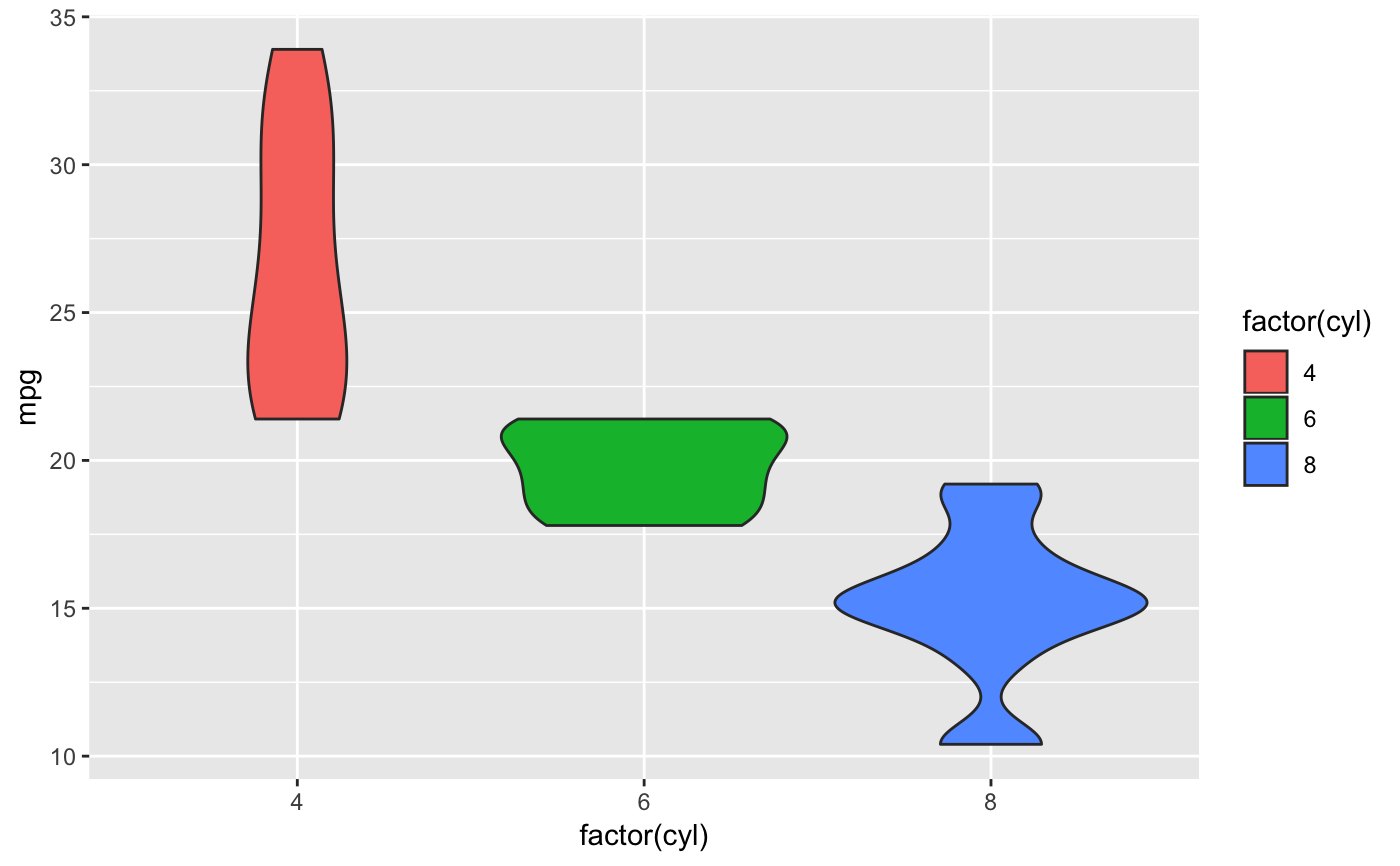
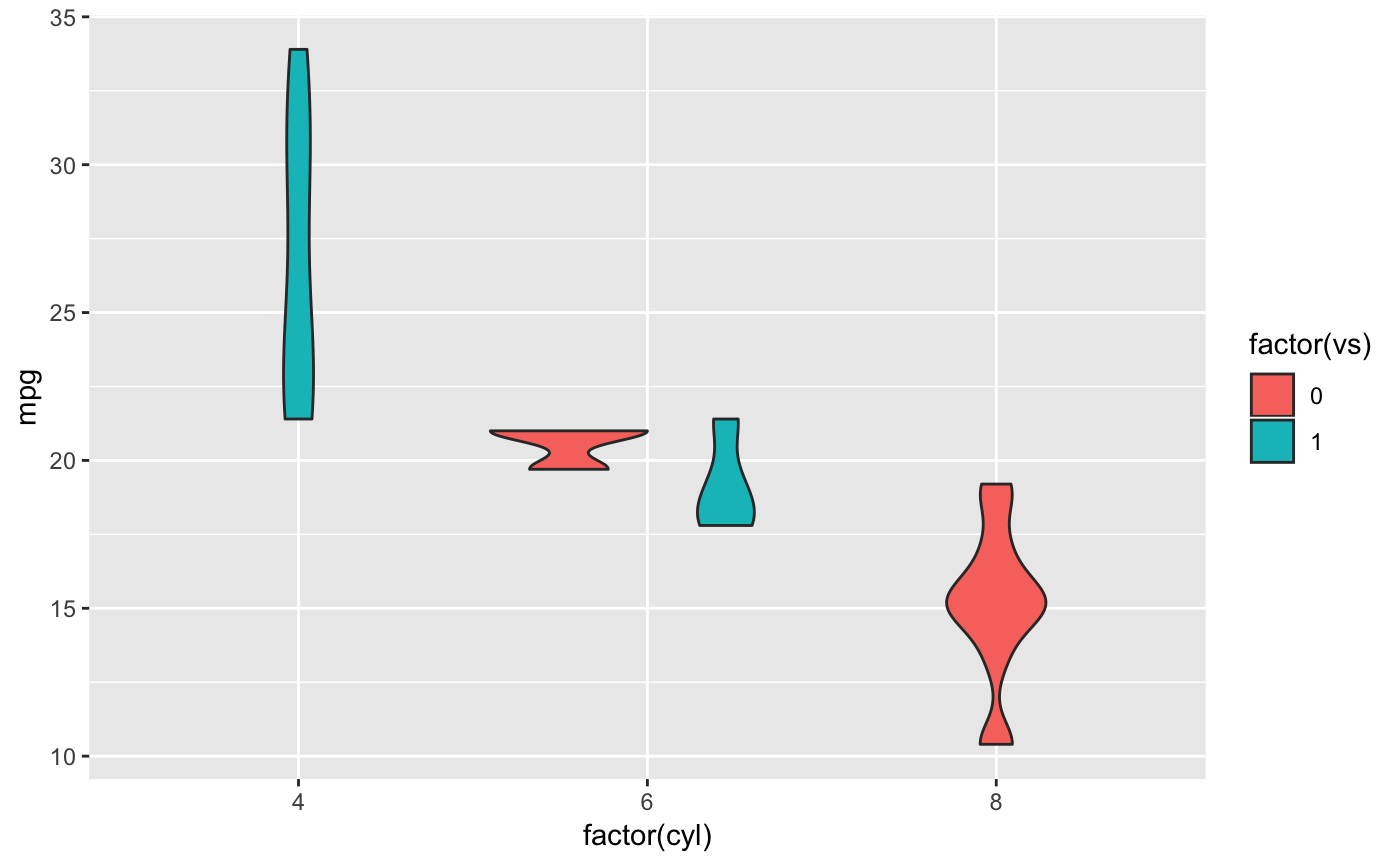
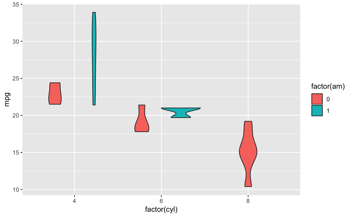
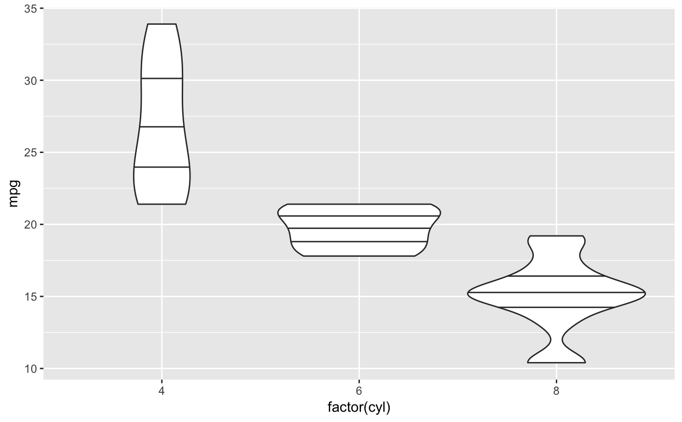
# Scale maximum width proportional to sample size:
p + geom_violin(scale = "count")

# Scale maximum width to 1 for all violins:
p + geom_violin(scale = "width")

# Default is to trim violins to the range of the data. To disable:
p + geom_violin(trim = FALSE)

# Use a smaller bandwidth for closer density fit (default is 1).
p + geom_violin(adjust = .5)

# Add aesthetic mappings
# Note that violins are automatically dodged when any aesthetic is
# a factor
p + geom_violin(aes(fill = cyl))
p + geom_violin(aes(fill = factor(cyl)))
p + geom_violin(aes(fill = factor(vs)))
p + geom_violin(aes(fill = factor(am)))

# Set aesthetics to fixed value
p + geom_violin(fill = "grey80", colour = "#3366FF")

# Show quartiles
p + geom_violin(draw_quantiles = c(0.25, 0.5, 0.75))

# Scales vs. coordinate transforms -------
if (require("ggplot2movies")) {
# Scale transformations occur before the density statistics are computed.
# Coordinate transformations occur afterwards.  Observe the effect on the
# number of outliers.
m <- ggplot(movies, aes(y = votes, x = rating, group = cut_width(rating, 0.5)))
m + geom_violin()
m + geom_violin() + scale_y_log10()
m + geom_violin() + coord_trans(y = "log10")
m + geom_violin() + scale_y_log10() + coord_trans(y = "log10")

# Violin plots with continuous x:
# Use the group aesthetic to group observations in violins
ggplot(movies, aes(year, budget)) + geom_violin()
ggplot(movies, aes(year, budget)) +
  geom_violin(aes(group = cut_width(year, 10)), scale = "width")
}
#> Warning: Removed 53573 rows containing non-finite values (stat_ydensity).