2d contours of a 3d surface

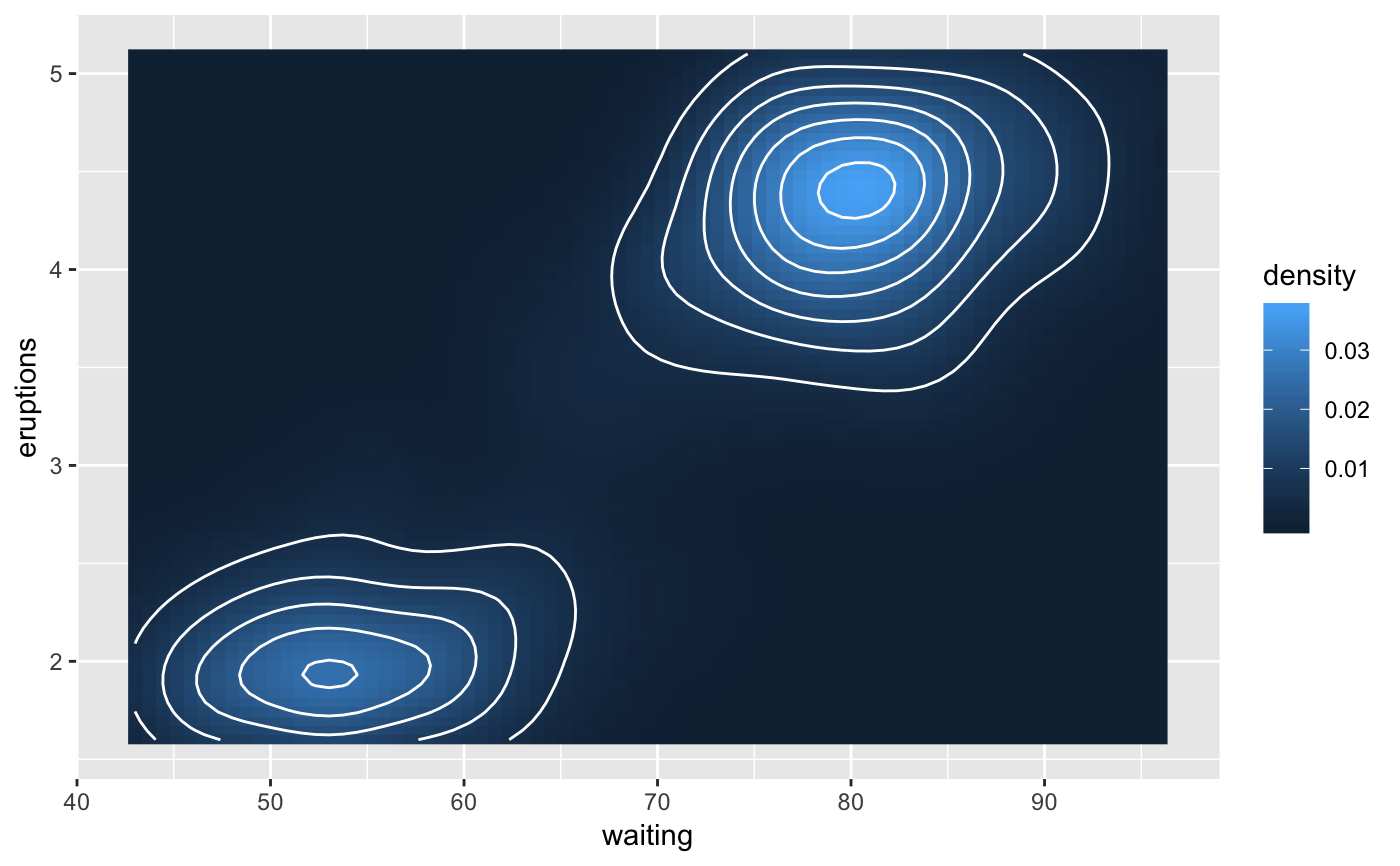
ggplot2 can not draw true 3d surfaces, but you can use geom_contour and geom_tile() to visualise 3d surfaces in 2d. To be a valid surface, the data must contain only a single row for each unique combination of the variables mapped to the x and y aesthetics. Contouring tends to work best when x and y form a (roughly) evenly spaced grid. If your data is not evenly spaced, you may want to interpolate to a grid before visualising.

geom_contour(mapping = NULL, data = NULL, stat = "contour",
  position = "identity", ..., lineend = "butt", linejoin = "round",
  linemitre = 10, na.rm = FALSE, show.legend = NA, inherit.aes = TRUE)

stat_contour(mapping = NULL, data = NULL, geom = "contour",
  position = "identity", ..., na.rm = FALSE, show.legend = NA,
  inherit.aes = TRUE)

Arguments

mapping	Set of aesthetic mappings created by aes() or aes_(). If specified and inherit.aes = TRUE (the default), it is combined with the default mapping at the top level of the plot. You must supply mapping if there is no plot mapping.
data	The data to be displayed in this layer. There are three options: If NULL, the default, the data is inherited from the plot data as specified in the call to ggplot(). A data.frame, or other object, will override the plot data. All objects will be fortified to produce a data frame. See fortify() for which variables will be created. A function will be called with a single argument, the plot data. The return value must be a data.frame., and will be used as the layer data.
stat	The statistical transformation to use on the data for this layer, as a string.
position	Position adjustment, either as a string, or the result of a call to a position adjustment function.
...	Other arguments passed on to layer(). These are often aesthetics, used to set an aesthetic to a fixed value, like color = "red" or size = 3. They may also be parameters to the paired geom/stat.
lineend	Line end style (round, butt, square).
linejoin	Line join style (round, mitre, bevel).
linemitre	Line mitre limit (number greater than 1).
na.rm	If FALSE, the default, missing values are removed with a warning. If TRUE, missing values are silently removed.
show.legend	logical. Should this layer be included in the legends? NA, the default, includes if any aesthetics are mapped. FALSE never includes, and TRUE always includes. It can also be a named logical vector to finely select the aesthetics to display.
inherit.aes	If FALSE, overrides the default aesthetics, rather than combining with them. This is most useful for helper functions that define both data and aesthetics and shouldn't inherit behaviour from the default plot specification, e.g. borders().
geom	The geometric object to use display the data

Aesthetics

geom_contour understands the following aesthetics (required aesthetics are in bold):

• x

• y

• alpha

• colour

• group

• linetype

• size

• weight

Learn more about setting these aesthetics in vignette("ggplot2-specs")

Computed variables

level

height of contour

See also

geom_density_2d(): 2d density contours

Examples

#' # Basic plot
v <- ggplot(faithfuld, aes(waiting, eruptions, z = density))
v + geom_contour()

# Or compute from raw data
ggplot(faithful, aes(waiting, eruptions)) +
  geom_density_2d()

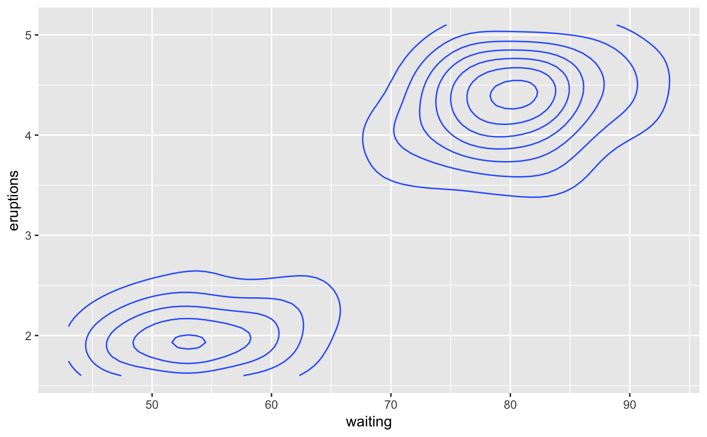
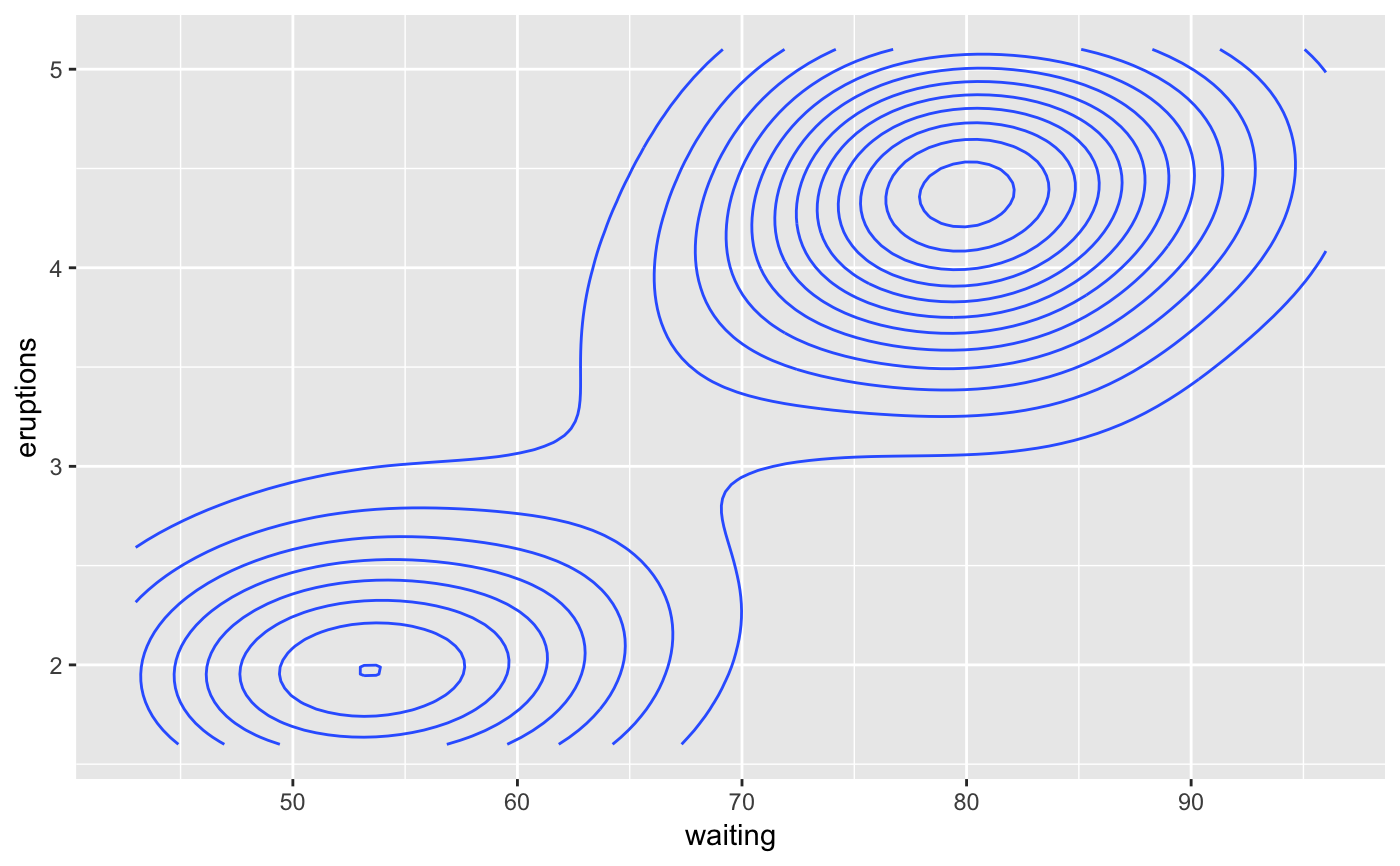
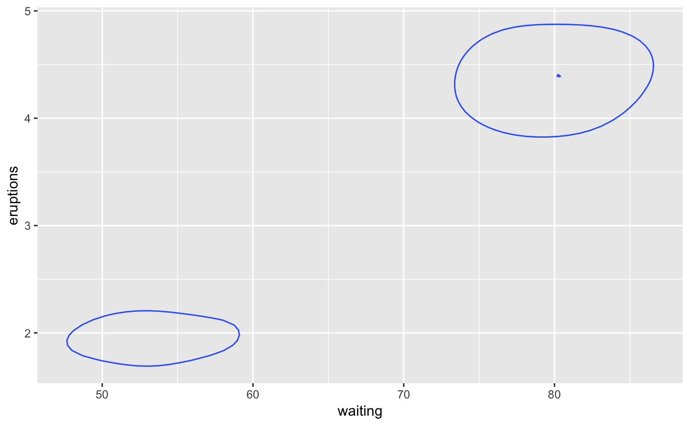
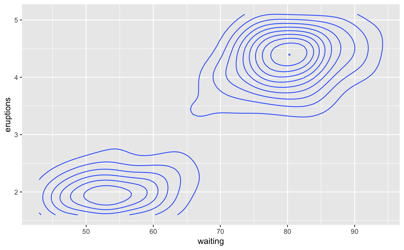
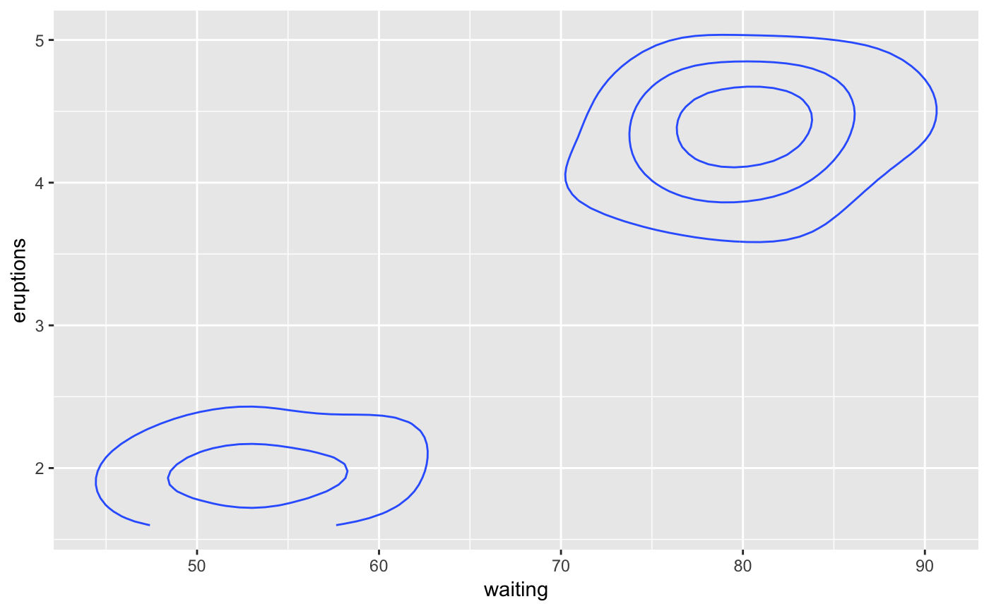
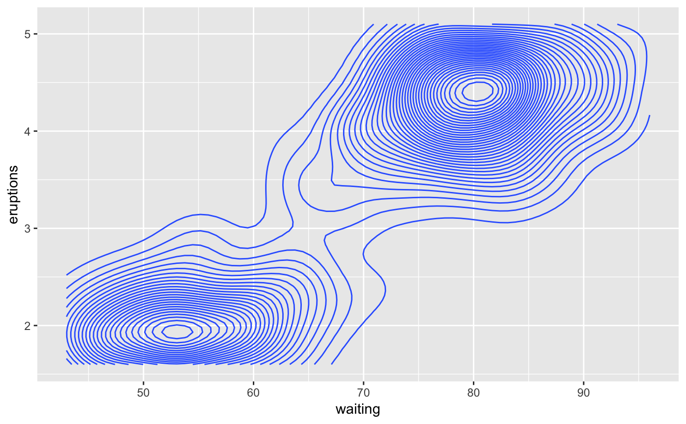
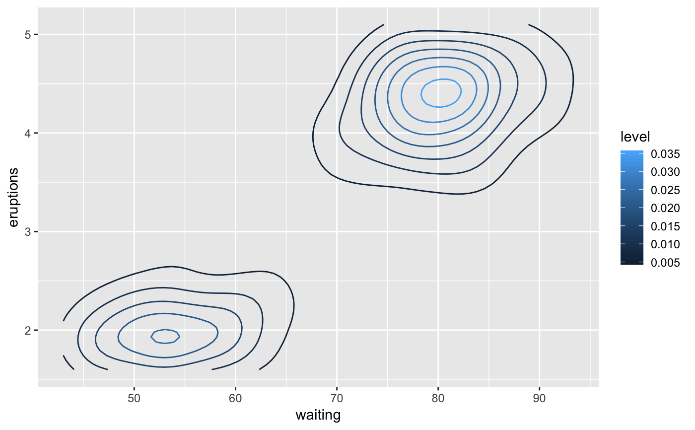
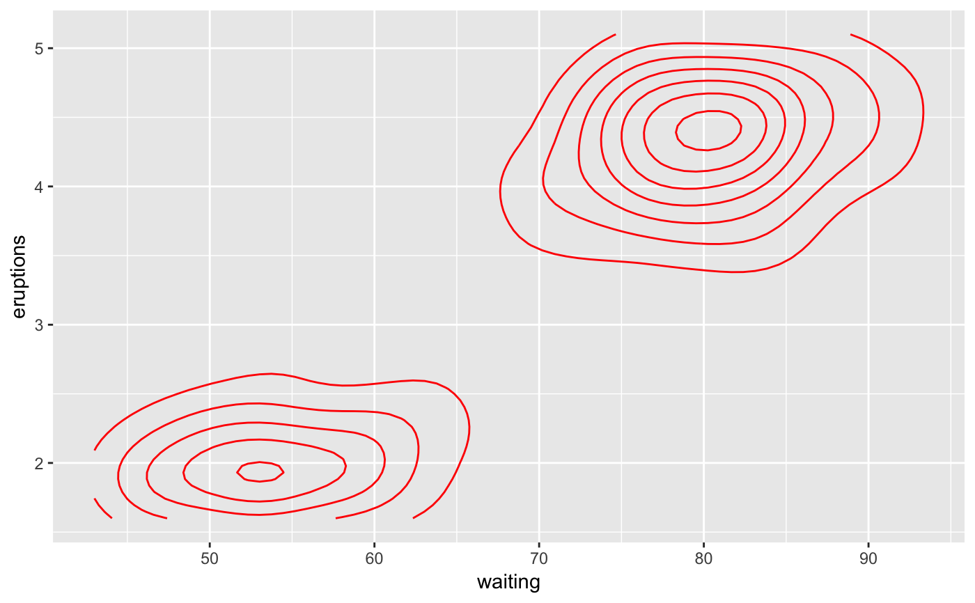
# Setting bins creates evenly spaced contours in the range of the data
v + geom_contour(bins = 2)
v + geom_contour(bins = 10)

# Setting binwidth does the same thing, parameterised by the distance
# between contours
v + geom_contour(binwidth = 0.01)
v + geom_contour(binwidth = 0.001)

# Other parameters
v + geom_contour(aes(colour = stat(level)))
v + geom_contour(colour = "red")
v + geom_raster(aes(fill = density)) +
  geom_contour(colour = "white")