Histograms and frequency polygons

Visualise the distribution of a single continuous variable by dividing the x axis into bins and counting the number of observations in each bin. Histograms (geom_histogram) display the count with bars; frequency polygons (geom_freqpoly) display the counts with lines. Frequency polygons are more suitable when you want to compare the distribution across the levels of a categorical variable.

geom_freqpoly(mapping = NULL, data = NULL, stat = "bin",
  position = "identity", ..., na.rm = FALSE, show.legend = NA,
  inherit.aes = TRUE)

geom_histogram(mapping = NULL, data = NULL, stat = "bin",
  position = "stack", ..., binwidth = NULL, bins = NULL, na.rm = FALSE,
  show.legend = NA, inherit.aes = TRUE)

stat_bin(mapping = NULL, data = NULL, geom = "bar", position = "stack",
  ..., binwidth = NULL, bins = NULL, center = NULL, boundary = NULL,
  breaks = NULL, closed = c("right", "left"), pad = FALSE,
  na.rm = FALSE, show.legend = NA, inherit.aes = TRUE)

Arguments

mapping	Set of aesthetic mappings created by aes() or aes_(). If specified and inherit.aes = TRUE (the default), it is combined with the default mapping at the top level of the plot. You must supply mapping if there is no plot mapping.
data	The data to be displayed in this layer. There are three options: If NULL, the default, the data is inherited from the plot data as specified in the call to ggplot(). A data.frame, or other object, will override the plot data. All objects will be fortified to produce a data frame. See fortify() for which variables will be created. A function will be called with a single argument, the plot data. The return value must be a data.frame., and will be used as the layer data.
position	Position adjustment, either as a string, or the result of a call to a position adjustment function.
...	Other arguments passed on to layer(). These are often aesthetics, used to set an aesthetic to a fixed value, like color = "red" or size = 3. They may also be parameters to the paired geom/stat.
na.rm	If FALSE, the default, missing values are removed with a warning. If TRUE, missing values are silently removed.
show.legend	logical. Should this layer be included in the legends? NA, the default, includes if any aesthetics are mapped. FALSE never includes, and TRUE always includes. It can also be a named logical vector to finely select the aesthetics to display.
inherit.aes	If FALSE, overrides the default aesthetics, rather than combining with them. This is most useful for helper functions that define both data and aesthetics and shouldn't inherit behaviour from the default plot specification, e.g. borders().
binwidth	The width of the bins. Can be specified as a numeric value, or a function that calculates width from x. The default is to use bins bins that cover the range of the data. You should always override this value, exploring multiple widths to find the best to illustrate the stories in your data. The bin width of a date variable is the number of days in each time; the bin width of a time variable is the number of seconds.
bins	Number of bins. Overridden by binwidth. Defaults to 30.
geom, stat	Use to override the default connection between geom_histogram/geom_freqpoly and stat_bin.
center	The center of one of the bins. Note that if center is above or below the range of the data, things will be shifted by an appropriate number of widths. To center on integers, for example, use width = 1 and center = 0, even if 0 is outside the range of the data. At most one of center and boundary may be specified.
boundary	A boundary between two bins. As with center, things are shifted when boundary is outside the range of the data. For example, to center on integers, use width = 1 and boundary = 0.5, even if 0.5 is outside the range of the data. At most one of center and boundary may be specified.
breaks	Alternatively, you can supply a numeric vector giving the bin boundaries. Overrides binwidth, bins, center, and boundary.
closed	One of "right" or "left" indicating whether right or left edges of bins are included in the bin.
pad	If TRUE, adds empty bins at either end of x. This ensures frequency polygons touch 0. Defaults to FALSE.

Details

stat_bin is suitable only for continuous x data. If your x data is discrete, you probably want to use stat_count().

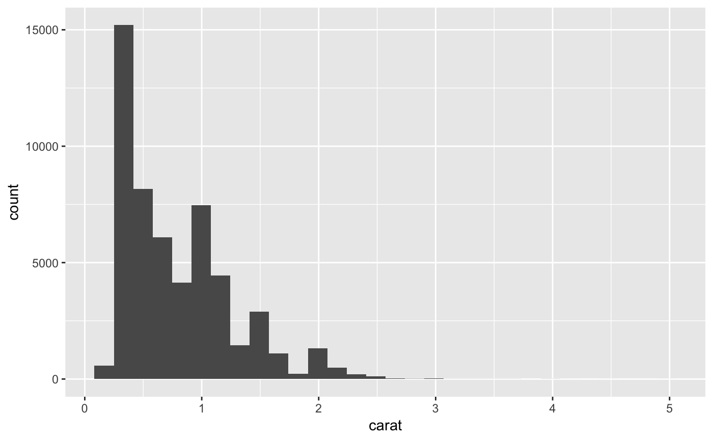
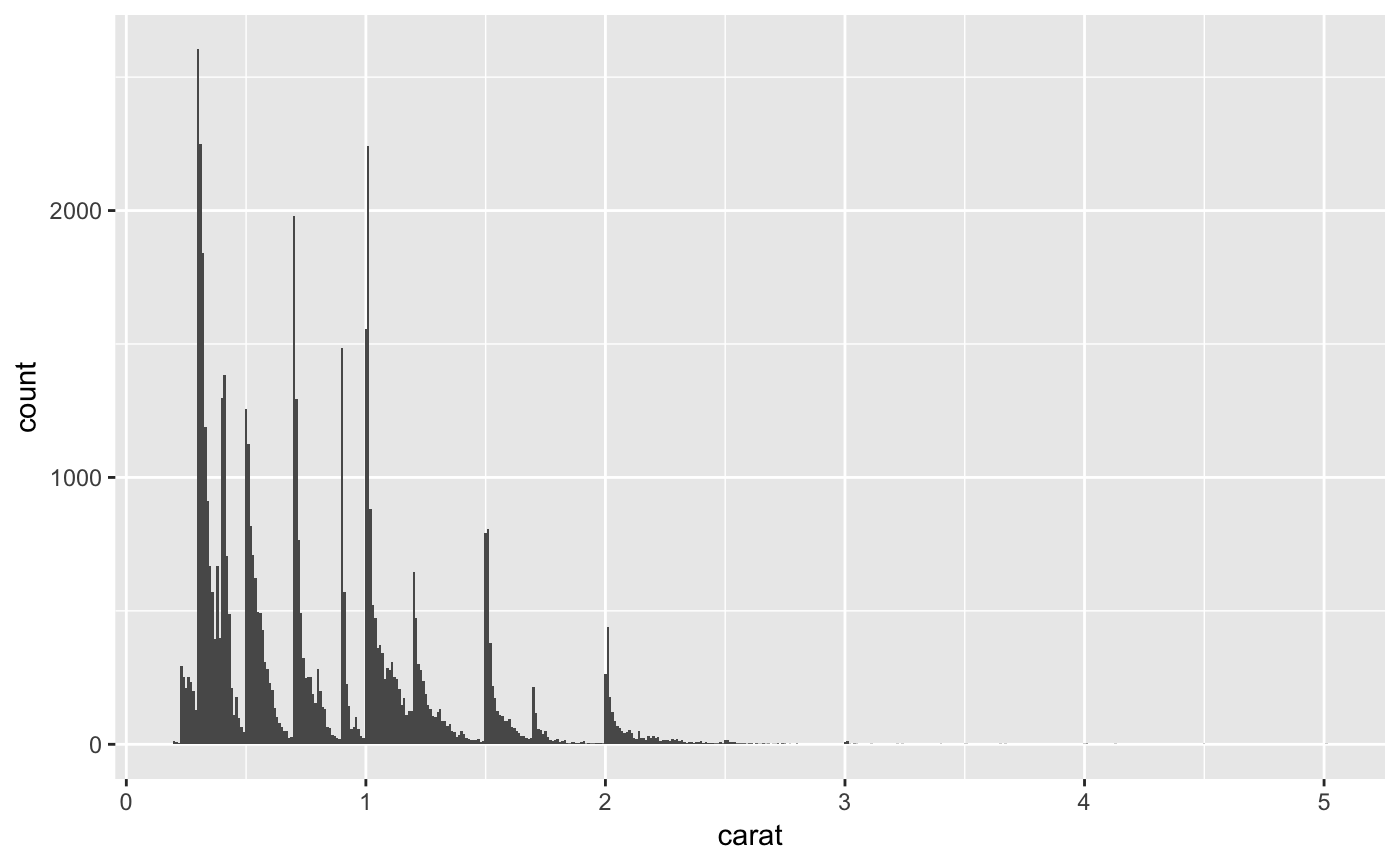
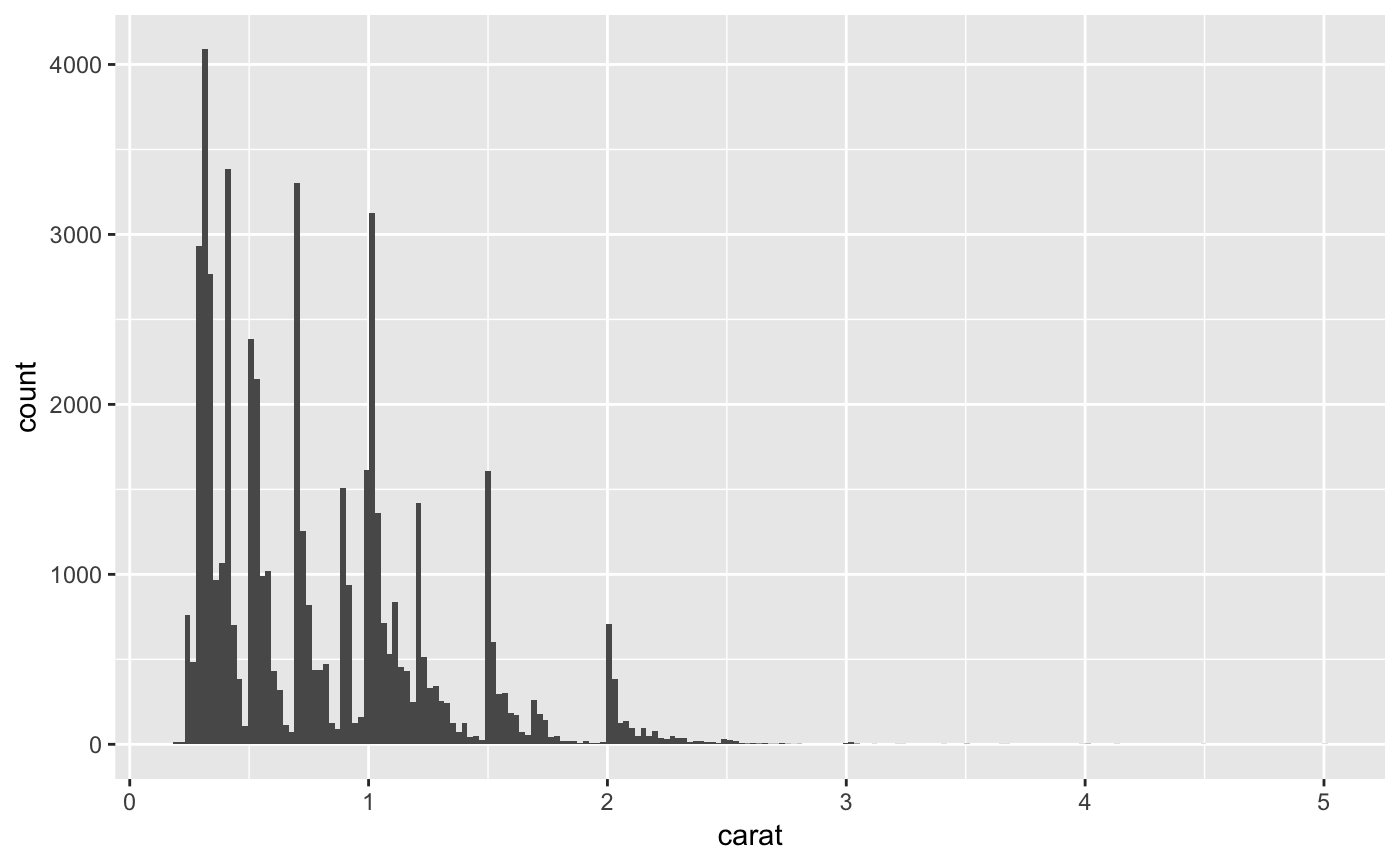
By default, the underlying computation (stat_bin) uses 30 bins; this is not a good default, but the idea is to get you experimenting with different bin widths. You may need to look at a few to uncover the full story behind your data.

Aesthetics

geom_histogram uses the same aesthetics as geom_bar(); geom_freqpoly uses the same aesthetics as geom_line().

Computed variables

count

number of points in bin

density

density of points in bin, scaled to integrate to 1

ncount

count, scaled to maximum of 1

ndensity

density, scaled to maximum of 1

See also

stat_count(), which counts the number of cases at each x position, without binning. It is suitable for both discrete and continuous x data, whereas stat_bin is suitable only for continuous x data.

Examples

ggplot(diamonds, aes(carat)) +
  geom_histogram()
#> `stat_bin()` using `bins = 30`. Pick better value with `binwidth`.
ggplot(diamonds, aes(carat)) +
  geom_histogram(binwidth = 0.01)
ggplot(diamonds, aes(carat)) +
  geom_histogram(bins = 200)

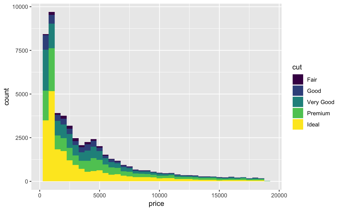
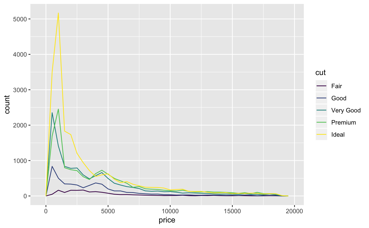
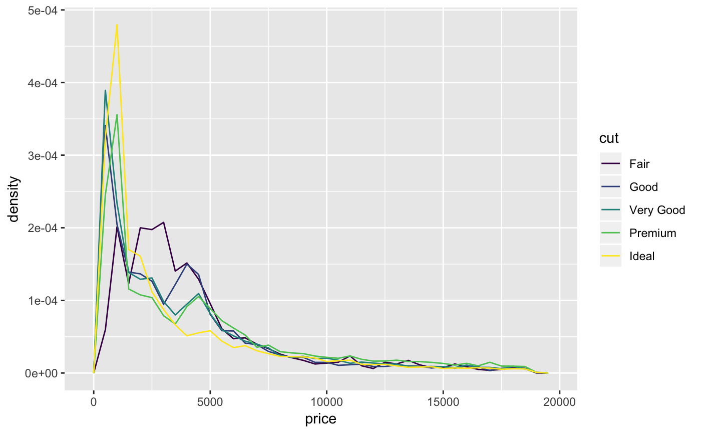
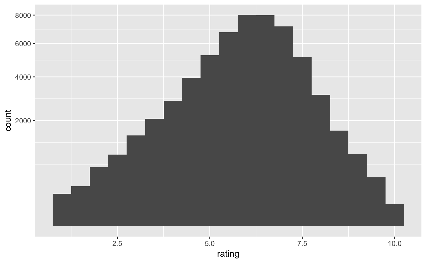
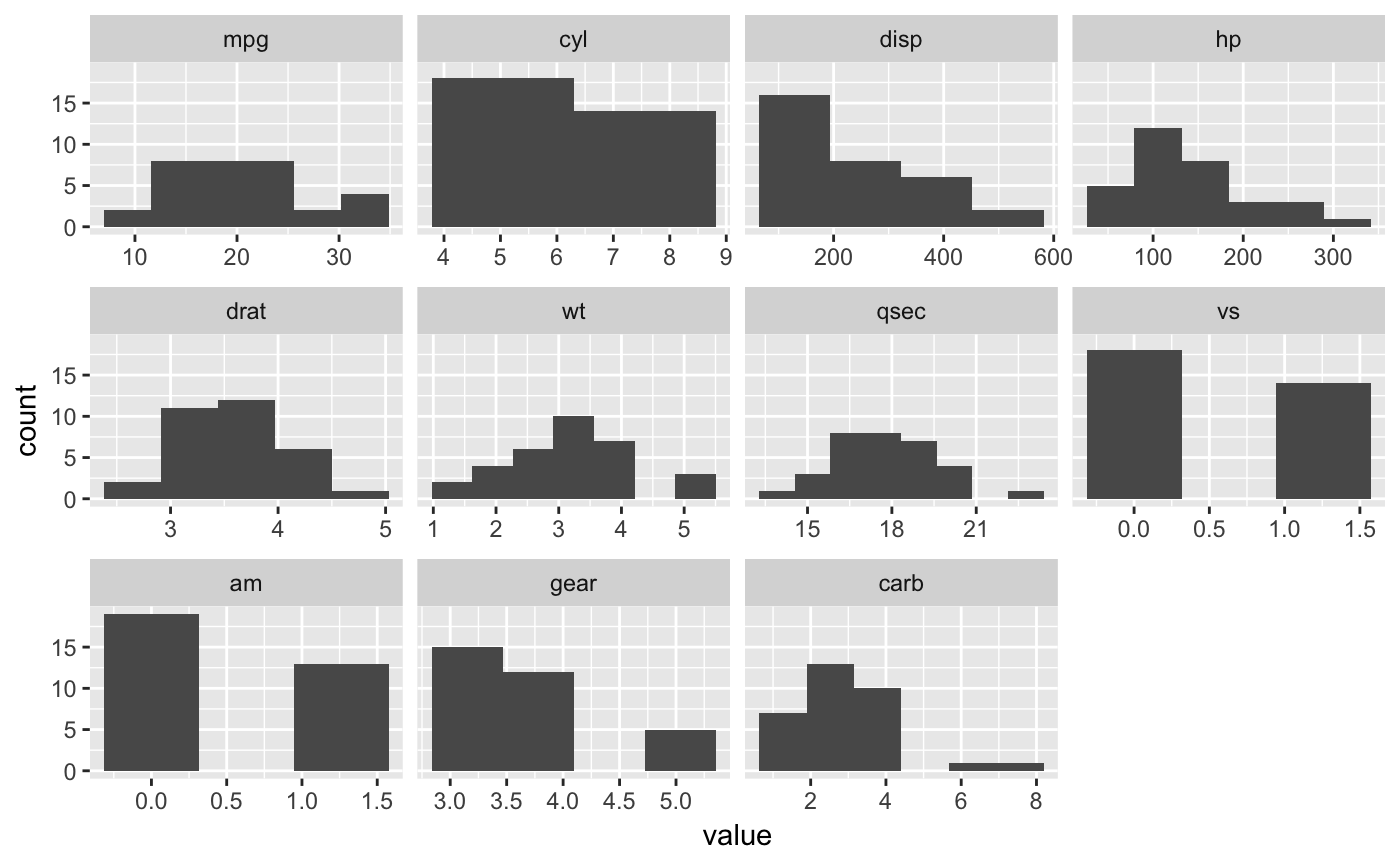
# Rather than stacking histograms, it's easier to compare frequency
# polygons
ggplot(diamonds, aes(price, fill = cut)) +
  geom_histogram(binwidth = 500)
ggplot(diamonds, aes(price, colour = cut)) +
  geom_freqpoly(binwidth = 500)

# To make it easier to compare distributions with very different counts,
# put density on the y axis instead of the default count
ggplot(diamonds, aes(price, stat(density), colour = cut)) +
  geom_freqpoly(binwidth = 500)

if (require("ggplot2movies")) {
# Often we don't want the height of the bar to represent the
# count of observations, but the sum of some other variable.
# For example, the following plot shows the number of movies
# in each rating.
m <- ggplot(movies, aes(rating))
m + geom_histogram(binwidth = 0.1)

# If, however, we want to see the number of votes cast in each
# category, we need to weight by the votes variable
m + geom_histogram(aes(weight = votes), binwidth = 0.1) + ylab("votes")

# For transformed scales, binwidth applies to the transformed data.
# The bins have constant width on the transformed scale.
m + geom_histogram() + scale_x_log10()
m + geom_histogram(binwidth = 0.05) + scale_x_log10()

# For transformed coordinate systems, the binwidth applies to the
# raw data. The bins have constant width on the original scale.

# Using log scales does not work here, because the first
# bar is anchored at zero, and so when transformed becomes negative
# infinity. This is not a problem when transforming the scales, because
# no observations have 0 ratings.
m + geom_histogram(boundary = 0) + coord_trans(x = "log10")
# Use boundary = 0, to make sure we don't take sqrt of negative values
m + geom_histogram(boundary = 0) + coord_trans(x = "sqrt")

# You can also transform the y axis.  Remember that the base of the bars
# has value 0, so log transformations are not appropriate
m <- ggplot(movies, aes(x = rating))
m + geom_histogram(binwidth = 0.5) + scale_y_sqrt()
}

# You can specify a function for calculating binwidth,
# particularly useful when faceting along variables with
# different ranges
mtlong <- reshape2::melt(mtcars)
#> No id variables; using all as measure variables
ggplot(mtlong, aes(value)) + facet_wrap(~variable, scales = 'free_x') +
  geom_histogram(binwidth = function(x) 2 * IQR(x) / (length(x)^(1/3)))