Aesthetics: grouping

Aesthetics: grouping

Examples

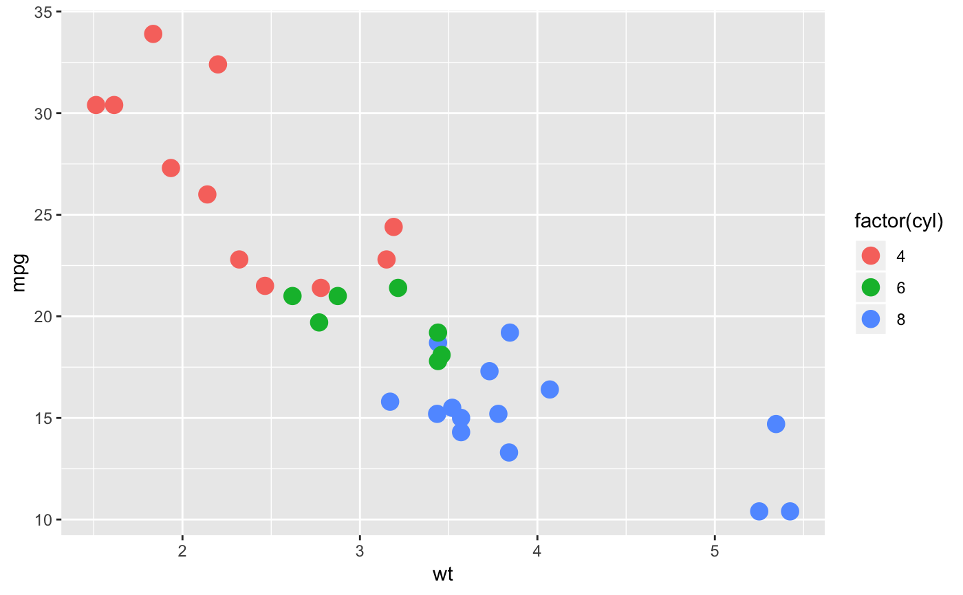
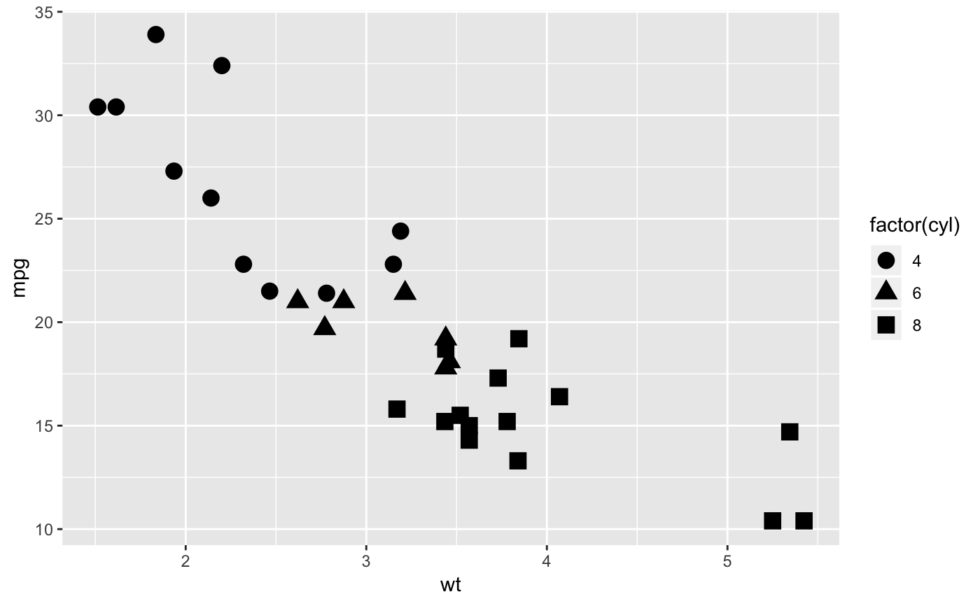
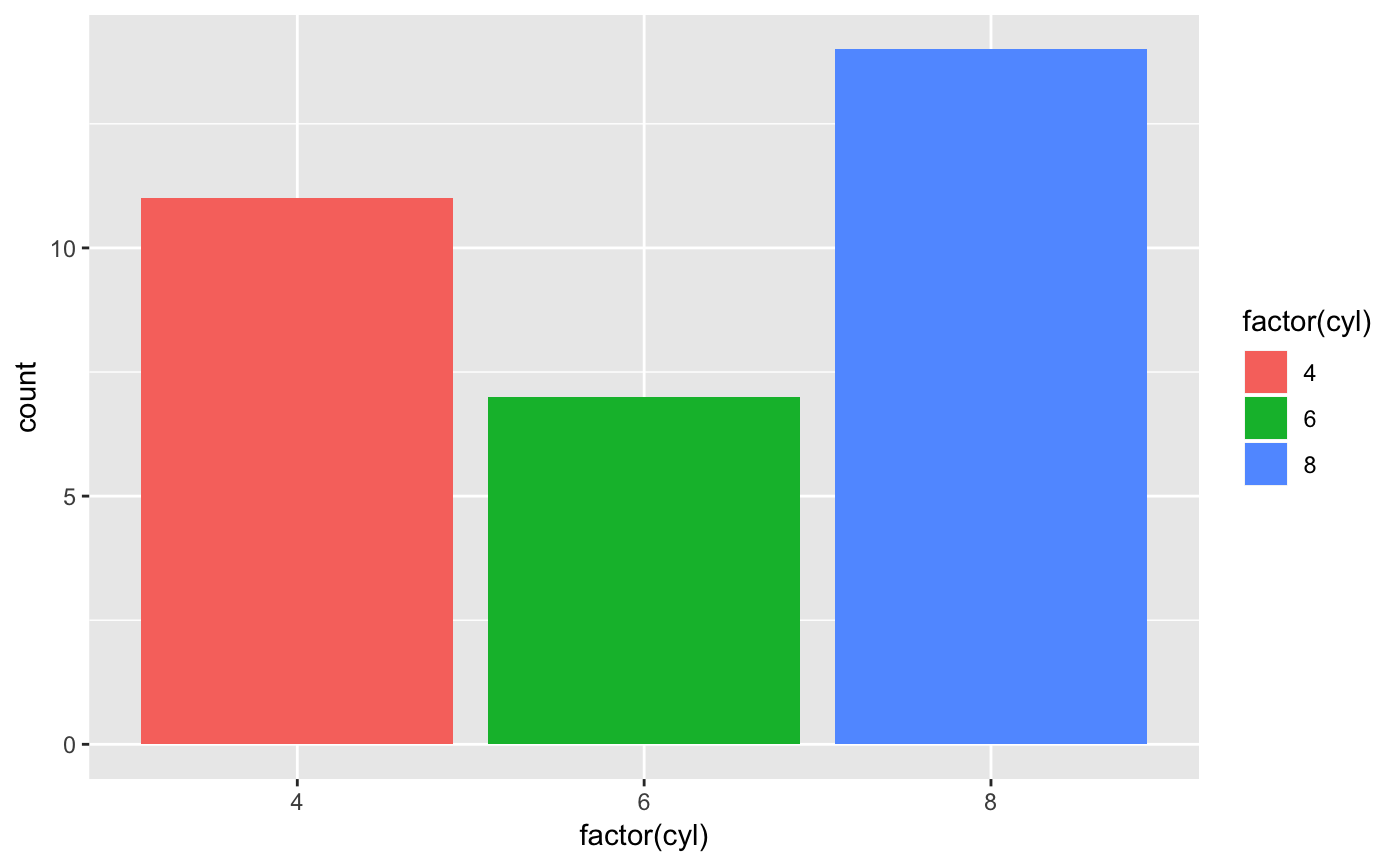
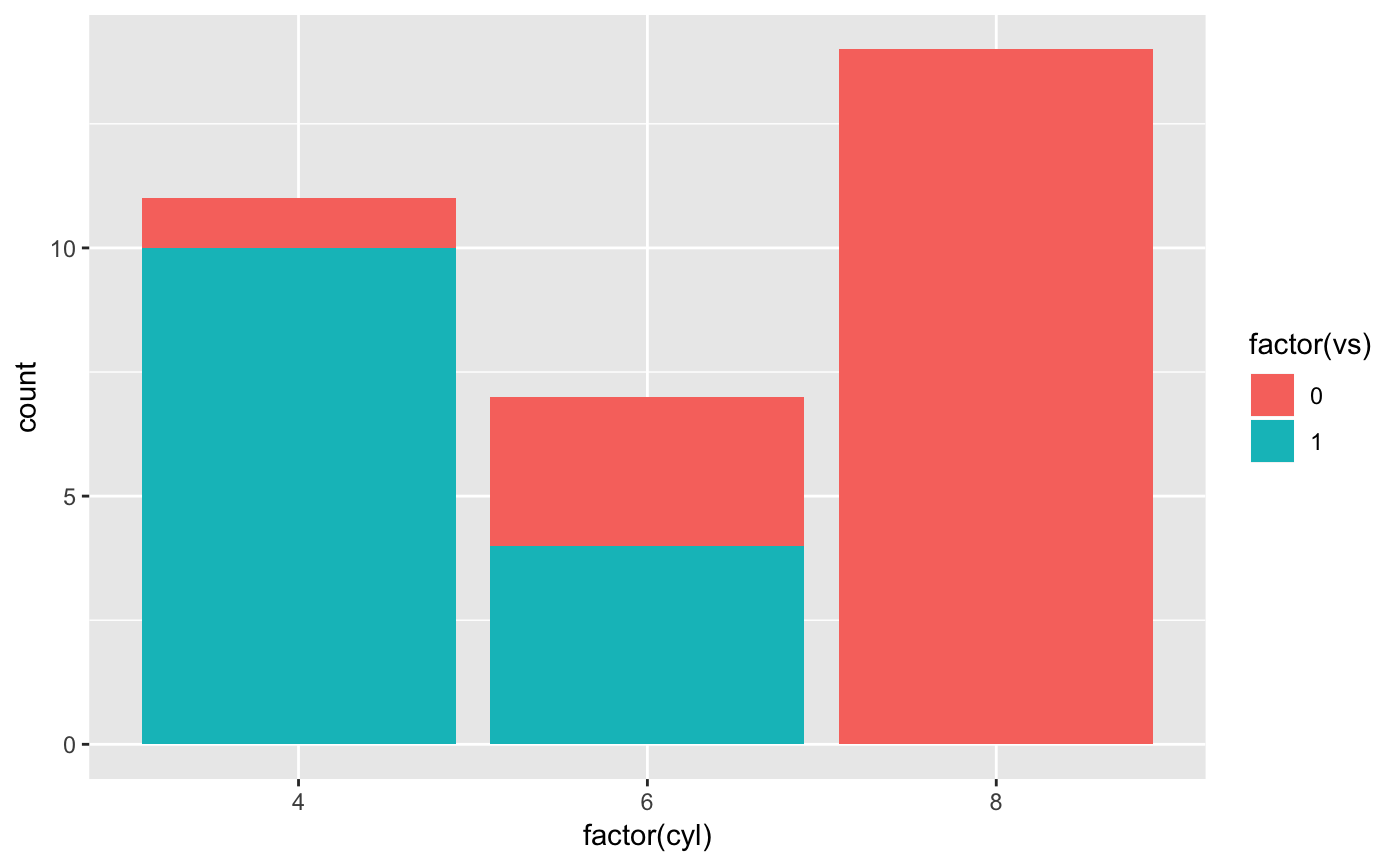
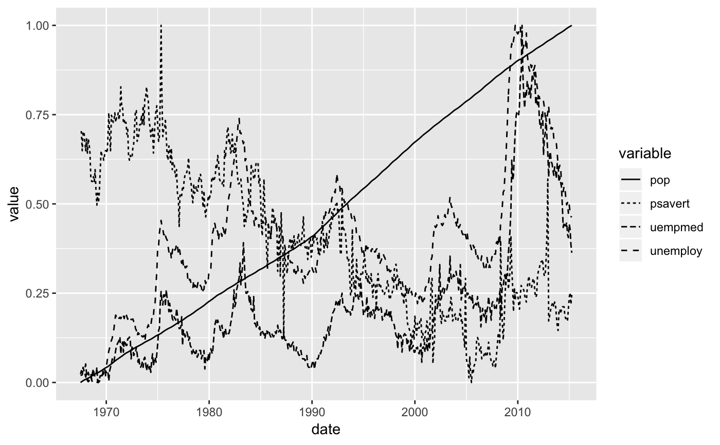
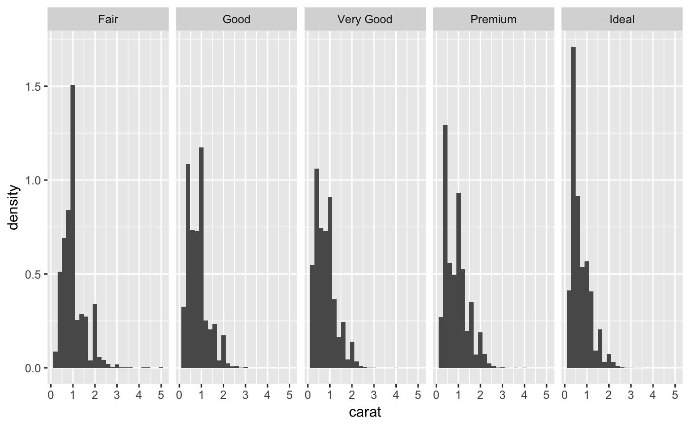
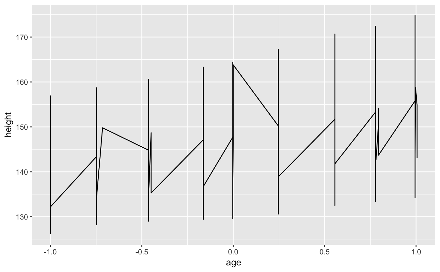
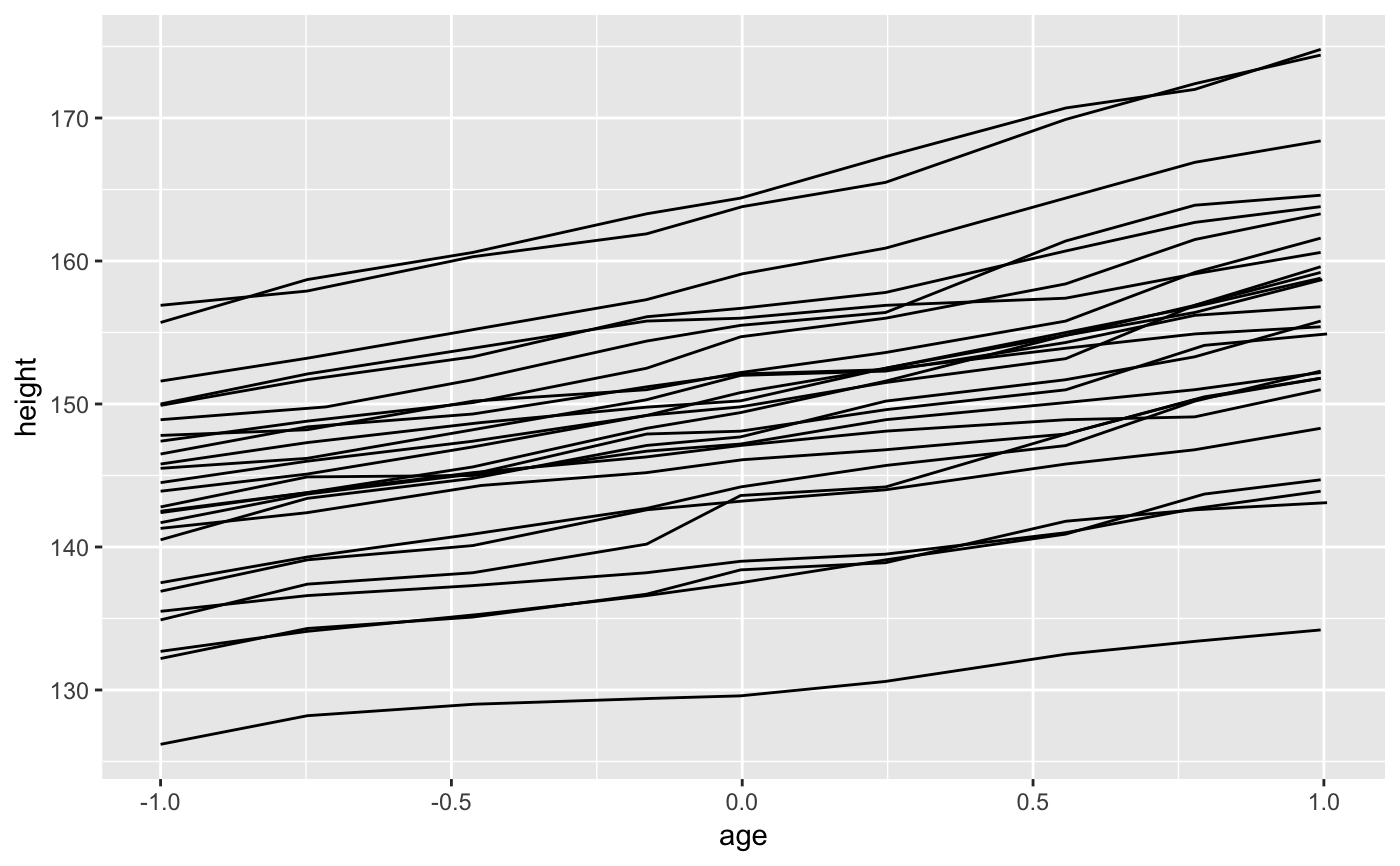
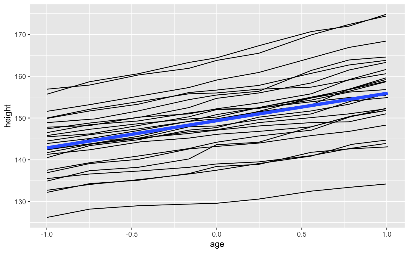
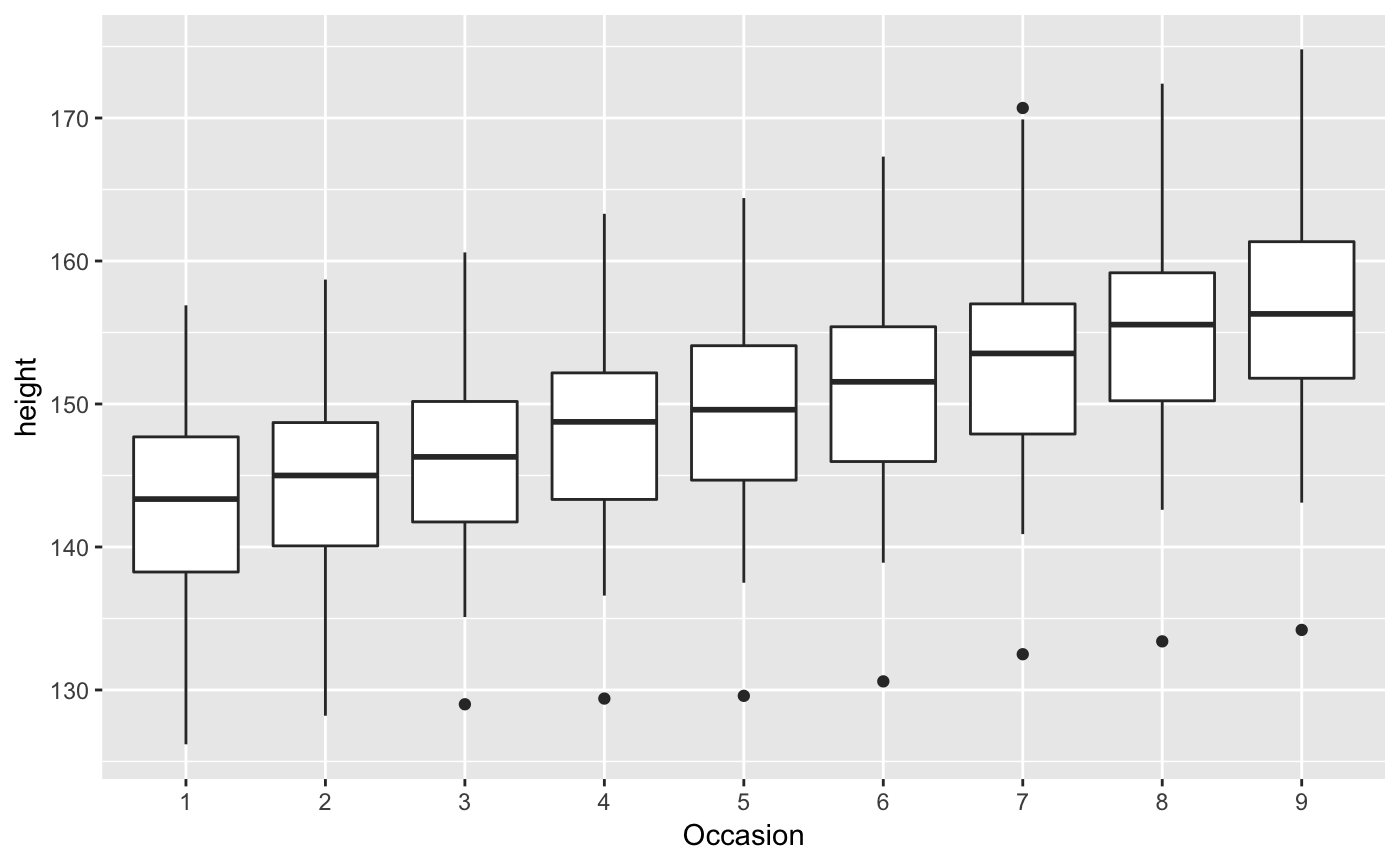
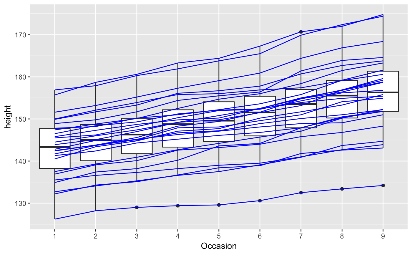
# By default, the group is set to the interaction of all discrete variables in the
# plot. This often partitions the data correctly, but when it does not, or when
# no discrete variable is used in the plot, you will need to explicitly define the
# grouping structure, by mapping group to a variable that has a different value
# for each group.

# For most applications you can simply specify the grouping with
# various aesthetics (colour, shape, fill, linetype) or with facets.

p <- ggplot(mtcars, aes(wt, mpg))
# A basic scatter plot
p + geom_point(size = 4)
# The colour aesthetic
p + geom_point(aes(colour = factor(cyl)), size = 4)
# Or you can use shape to distinguish the data
p + geom_point(aes(shape = factor(cyl)), size = 4)

# Using fill
a <- ggplot(mtcars, aes(factor(cyl)))
a + geom_bar()
a + geom_bar(aes(fill = factor(cyl)))
a + geom_bar(aes(fill = factor(vs)))

# Using linetypes
rescale01 <- function(x) (x - min(x)) / diff(range(x))
ec_scaled <- data.frame(
  date = economics$date,
  plyr::colwise(rescale01)(economics[, -(1:2)]))
ecm <- reshape2::melt(ec_scaled, id.vars = "date")
f <- ggplot(ecm, aes(date, value))
f + geom_line(aes(linetype = variable))

# Using facets
k <- ggplot(diamonds, aes(carat, stat(density))) + geom_histogram(binwidth = 0.2)
k + facet_grid(. ~ cut)

# There are three common cases where the default is not enough, and we
# will consider each one below. In the following examples, we will use a simple
# longitudinal dataset, Oxboys, from the nlme package. It records the heights
# (height) and centered ages (age) of 26 boys (Subject), measured on nine
# occasions (Occasion).

# Multiple groups with one aesthetic
h <- ggplot(nlme::Oxboys, aes(age, height))
# A single line tries to connect all the observations
h + geom_line()
# The group aesthetic maps a different line for each subject
h + geom_line(aes(group = Subject))

# Different groups on different layers
h <- h + geom_line(aes(group = Subject))
# Using the group aesthetic with both geom_line() and geom_smooth()
# groups the data the same way for both layers
h + geom_smooth(aes(group = Subject), method = "lm", se = FALSE)
# Changing the group aesthetic for the smoother layer
# fits a single line of best fit across all boys
h + geom_smooth(aes(group = 1), size = 2, method = "lm", se = FALSE)

# Overriding the default grouping
# The plot has a discrete scale but you want to draw lines that connect across
# groups. This is the strategy used in interaction plots, profile plots, and parallel
# coordinate plots, among others. For example, we draw boxplots of height at
# each measurement occasion
boysbox <- ggplot(nlme::Oxboys, aes(Occasion, height))
boysbox + geom_boxplot()
# There is no need to specify the group aesthetic here; the default grouping
# works because occasion is a discrete variable. To overlay individual trajectories
# we again need to override the default grouping for that layer with aes(group = Subject)
boysbox <- boysbox + geom_boxplot()
boysbox + geom_line(aes(group = Subject), colour = "blue")