Summarise y values at unique/binned x

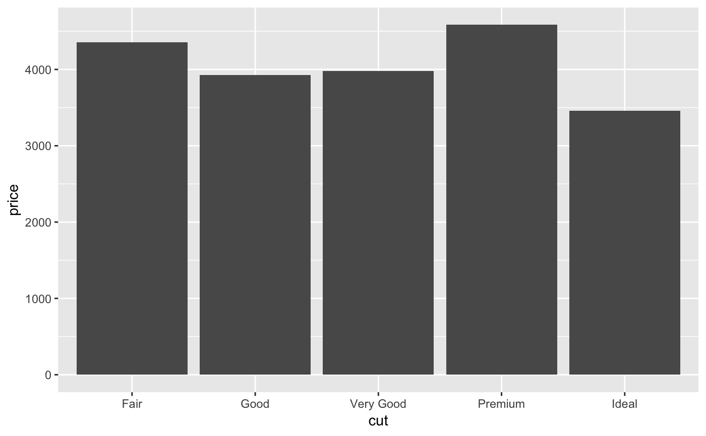
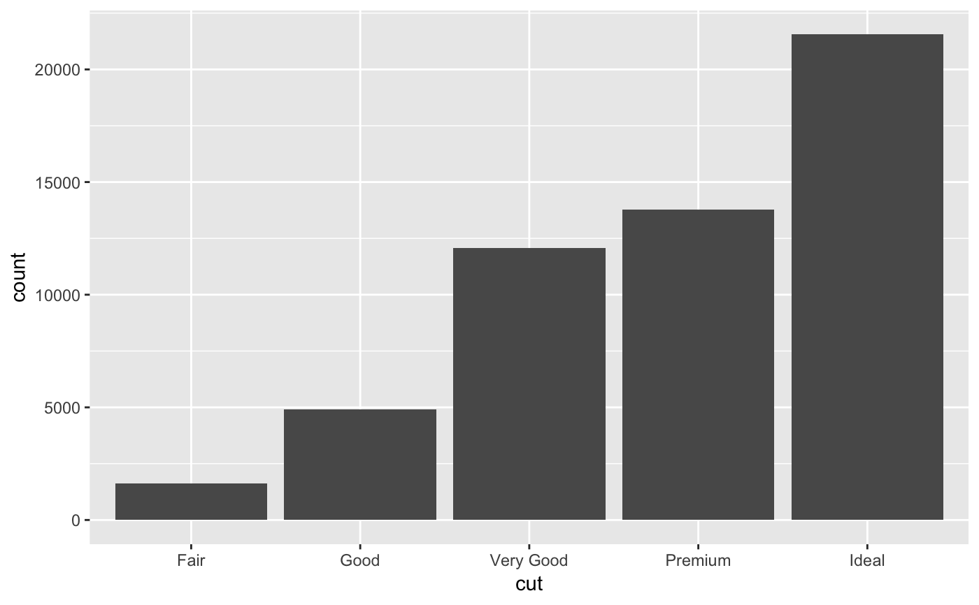
stat_summary operates on unique x; stat_summary_bin operates on binned x. They are more flexible versions of stat_bin(): instead of just counting, they can compute any aggregate.

stat_summary_bin(mapping = NULL, data = NULL, geom = "pointrange",
  position = "identity", ..., fun.data = NULL, fun.y = NULL,
  fun.ymax = NULL, fun.ymin = NULL, fun.args = list(), bins = 30,
  binwidth = NULL, breaks = NULL, na.rm = FALSE, show.legend = NA,
  inherit.aes = TRUE)

stat_summary(mapping = NULL, data = NULL, geom = "pointrange",
  position = "identity", ..., fun.data = NULL, fun.y = NULL,
  fun.ymax = NULL, fun.ymin = NULL, fun.args = list(), na.rm = FALSE,
  show.legend = NA, inherit.aes = TRUE)

Arguments

mapping	Set of aesthetic mappings created by aes() or aes_(). If specified and inherit.aes = TRUE (the default), it is combined with the default mapping at the top level of the plot. You must supply mapping if there is no plot mapping.
data	The data to be displayed in this layer. There are three options: If NULL, the default, the data is inherited from the plot data as specified in the call to ggplot(). A data.frame, or other object, will override the plot data. All objects will be fortified to produce a data frame. See fortify() for which variables will be created. A function will be called with a single argument, the plot data. The return value must be a data.frame., and will be used as the layer data.
geom	Use to override the default connection between geom_histogram/geom_freqpoly and stat_bin.
position	Position adjustment, either as a string, or the result of a call to a position adjustment function.
...	Other arguments passed on to layer(). These are often aesthetics, used to set an aesthetic to a fixed value, like color = "red" or size = 3. They may also be parameters to the paired geom/stat.
fun.data	A function that is given the complete data and should return a data frame with variables ymin, y, and ymax.
fun.ymin, fun.y, fun.ymax	Alternatively, supply three individual functions that are each passed a vector of x's and should return a single number.
fun.args	Optional additional arguments passed on to the functions.
bins	Number of bins. Overridden by binwidth. Defaults to 30.
binwidth	The width of the bins. Can be specified as a numeric value, or a function that calculates width from x. The default is to use bins bins that cover the range of the data. You should always override this value, exploring multiple widths to find the best to illustrate the stories in your data. The bin width of a date variable is the number of days in each time; the bin width of a time variable is the number of seconds.
breaks	Alternatively, you can supply a numeric vector giving the bin boundaries. Overrides binwidth, bins, center, and boundary.
na.rm	If FALSE, the default, missing values are removed with a warning. If TRUE, missing values are silently removed.
show.legend	logical. Should this layer be included in the legends? NA, the default, includes if any aesthetics are mapped. FALSE never includes, and TRUE always includes. It can also be a named logical vector to finely select the aesthetics to display.
inherit.aes	If FALSE, overrides the default aesthetics, rather than combining with them. This is most useful for helper functions that define both data and aesthetics and shouldn't inherit behaviour from the default plot specification, e.g. borders().

Aesthetics

stat_summary understands the following aesthetics (required aesthetics are in bold):

• x

• y

• group

Learn more about setting these aesthetics in vignette("ggplot2-specs")

Summary functions

You can either supply summary functions individually (fun.y, fun.ymax, fun.ymin), or as a single function (fun.data):

fun.data

Complete summary function. Should take numeric vector as input and return data frame as output

fun.ymin

ymin summary function (should take numeric vector and return single number)

fun.y

y summary function (should take numeric vector and return single number)

fun.ymax

ymax summary function (should take numeric vector and return single number)

A simple vector function is easiest to work with as you can return a single number, but is somewhat less flexible. If your summary function computes multiple values at once (e.g. ymin and ymax), use fun.data.

If no aggregation functions are suppled, will default to mean_se().

See also

geom_errorbar(), geom_pointrange(), geom_linerange(), geom_crossbar() for geoms to display summarised data

Examples

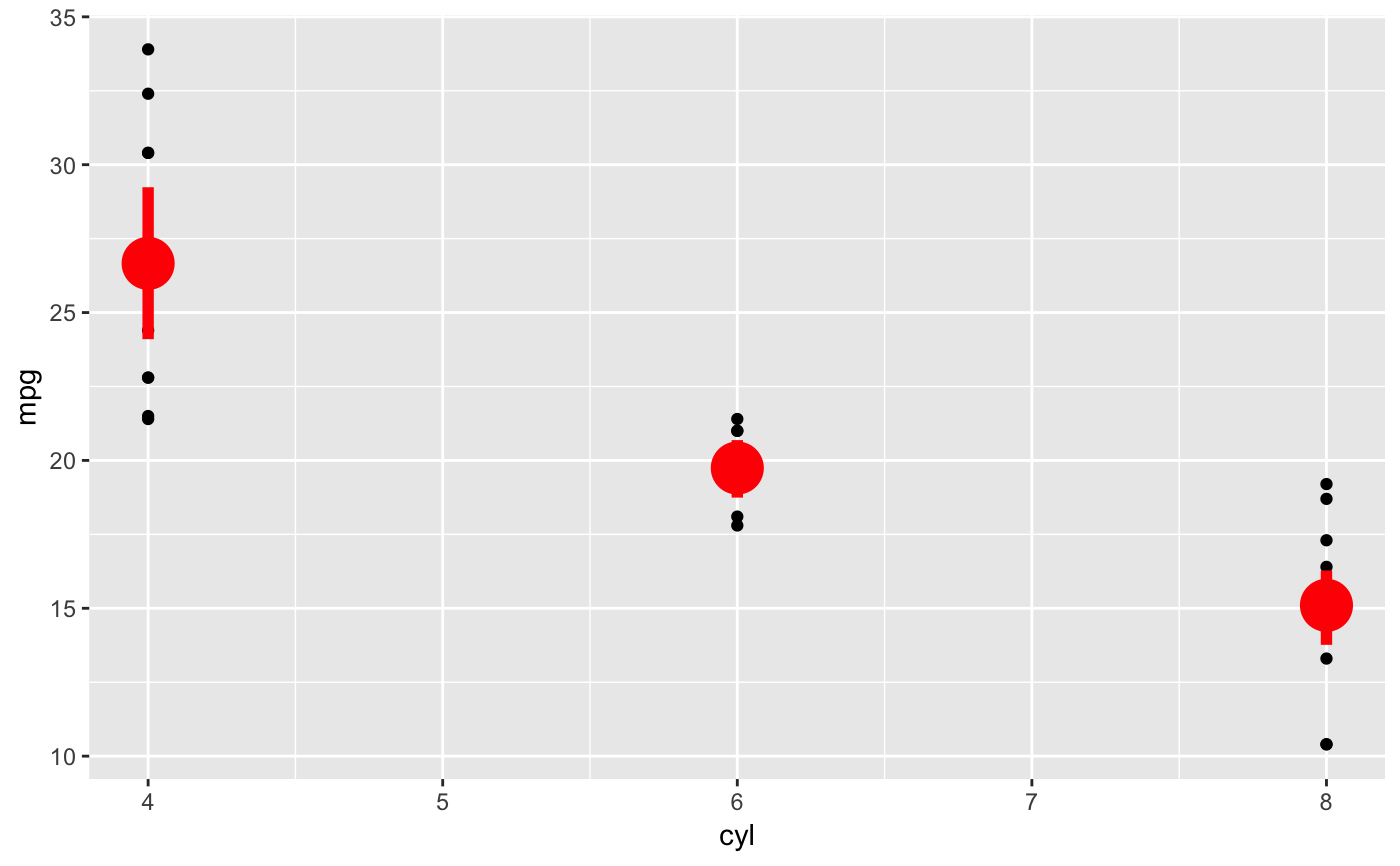
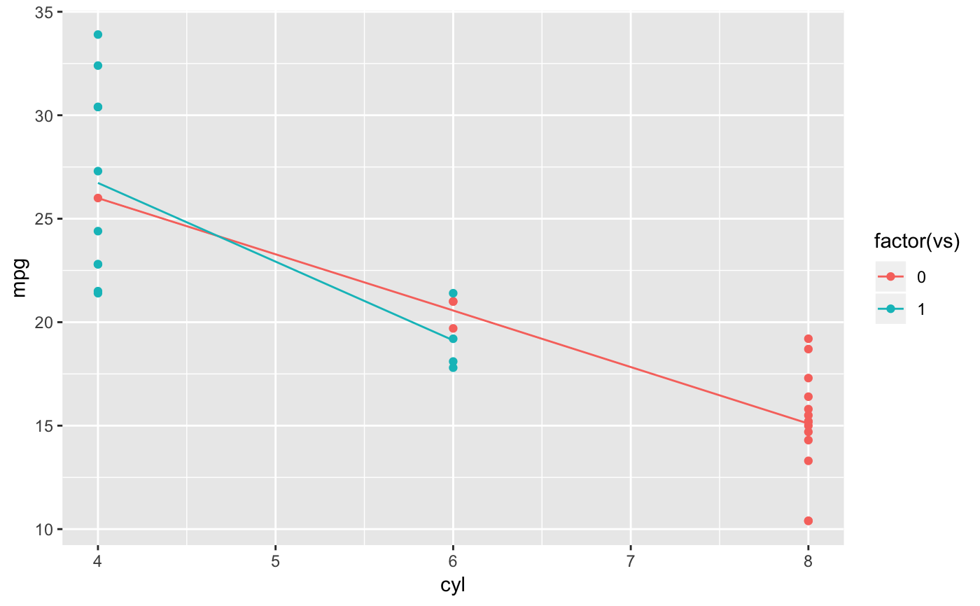
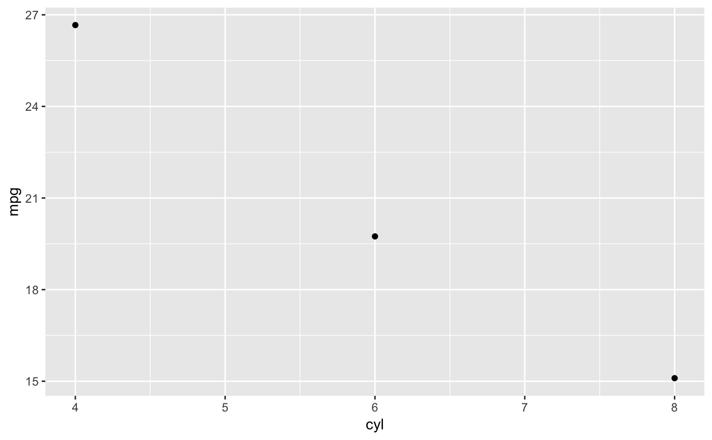
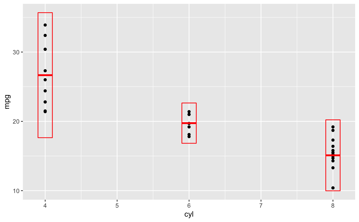
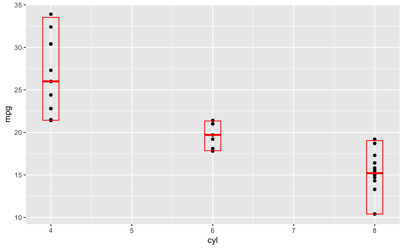
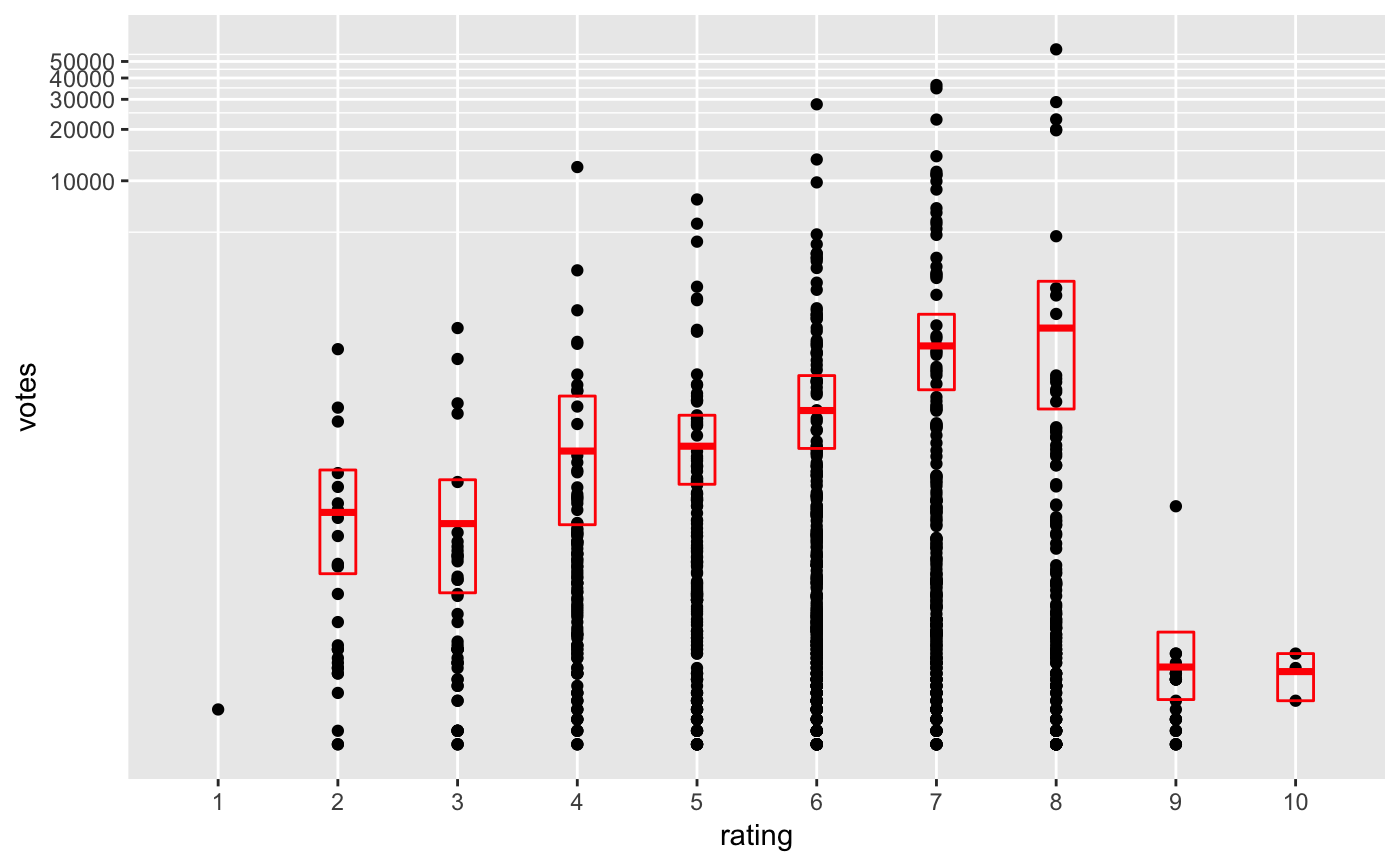
d <- ggplot(mtcars, aes(cyl, mpg)) + geom_point()
d + stat_summary(fun.data = "mean_cl_boot", colour = "red", size = 2)

# You can supply individual functions to summarise the value at
# each x:
d + stat_summary(fun.y = "median", colour = "red", size = 2, geom = "point")
d + stat_summary(fun.y = "mean", colour = "red", size = 2, geom = "point")
d + aes(colour = factor(vs)) + stat_summary(fun.y = mean, geom="line")

d + stat_summary(fun.y = mean, fun.ymin = min, fun.ymax = max,
  colour = "red")

d <- ggplot(diamonds, aes(cut))
d + geom_bar()
d + stat_summary_bin(aes(y = price), fun.y = "mean", geom = "bar")

# Don't use ylim to zoom into a summary plot - this throws the
# data away
p <- ggplot(mtcars, aes(cyl, mpg)) +
  stat_summary(fun.y = "mean", geom = "point")
p
p + ylim(15, 30)
#> Warning: Removed 9 rows containing non-finite values (stat_summary).
# Instead use coord_cartesian
p + coord_cartesian(ylim = c(15, 30))

# A set of useful summary functions is provided from the Hmisc package:
stat_sum_df <- function(fun, geom="crossbar", ...) {
  stat_summary(fun.data = fun, colour = "red", geom = geom, width = 0.2, ...)
}
d <- ggplot(mtcars, aes(cyl, mpg)) + geom_point()
# The crossbar geom needs grouping to be specified when used with
# a continuous x axis.
d + stat_sum_df("mean_cl_boot", mapping = aes(group = cyl))
d + stat_sum_df("mean_sdl", mapping = aes(group = cyl))
d + stat_sum_df("mean_sdl", fun.args = list(mult = 1), mapping = aes(group = cyl))
d + stat_sum_df("median_hilow", mapping = aes(group = cyl))

# An example with highly skewed distributions:
if (require("ggplot2movies")) {
set.seed(596)
mov <- movies[sample(nrow(movies), 1000), ]
 m2 <- ggplot(mov, aes(x = factor(round(rating)), y = votes)) + geom_point()
 m2 <- m2 + stat_summary(fun.data = "mean_cl_boot", geom = "crossbar",
                         colour = "red", width = 0.3) + xlab("rating")
m2
# Notice how the overplotting skews off visual perception of the mean
# supplementing the raw data with summary statistics is _very_ important

# Next, we'll look at votes on a log scale.

# Transforming the scale means the data are transformed
# first, after which statistics are computed:
m2 + scale_y_log10()
# Transforming the coordinate system occurs after the
# statistic has been computed. This means we're calculating the summary on the raw data
# and stretching the geoms onto the log scale.  Compare the widths of the
# standard errors.
m2 + coord_trans(y="log10")
}
#> Warning: Removed 1 rows containing missing values (geom_crossbar).